Mechanical Forex

Those of you who follow my articles in currency trader magazine might be familiar with an article I published last year in which I develop a new statistic to measure system quality called the ideal R (IR). This trading statistic uses the notion of what we would consider a “perfect system” and attempts to find how close a strategy is to this notion via the use of linear regressions. In essence what we want to know is how closely a system fits a perfect line with no drawdown (the ideal system) but in order to do so we must expand our search beyond the concept of a single simple linear regression, as this technique does not give us the best results in this regard (as linear regression models compensate for symmetric deviations from the regression line). Through this post I will show you how you can calculate the IR trading statistic using the R statistical software. If you’re not familiar with R I would recommend you to follow this link so that you can read some of my R related posts and tutorials. You will need quantmod and the performanceAnalytics library to perform this analysis.

–

–

When you try to find a system that is as stable as possible (similar results across a wide variety of market conditions), the idea of linear regression comes straight to mind. A non-compounding system with a linear return curve or a compounding system where the logarithm of the balance gives a linear return curve, are both examples of strategies that should give perfect linear results in the ideal case. Finding how strongly systems deviate from this ideal case will give you a good idea about how good or bad your trading strategy actually is. The way to approach this seems simple, if a strategy should fit a simple line, then a linear regression analysis should give us a good idea whether this is true or false. However the linear regression model has some problems as the fitting criteria converge exponentially towards perfect records as the curve looks more like the ideal case.

What does this mean? It means that as your system becomes more linear, the linear regression model will have trouble telling how different it is from an absolutely straight line, since the deviations across your system test will be both too small and too symmetrically compensated to draw any clear distinction. A system with an R^2 of 0.99 can still have substantial deviations from the ideal, perfect system, while the linear regression model predicts that it should be “almost perfect”. The problem lies in the way in which the linear regression calculates correlation coefficients and the way in which symmetric deviations are compensated within the model across a long sample that is of a fundamentally linear nature. The currency trader magazine article mentioned before contains some examples showing how the simple linear regression model becomes problematic at high R values.

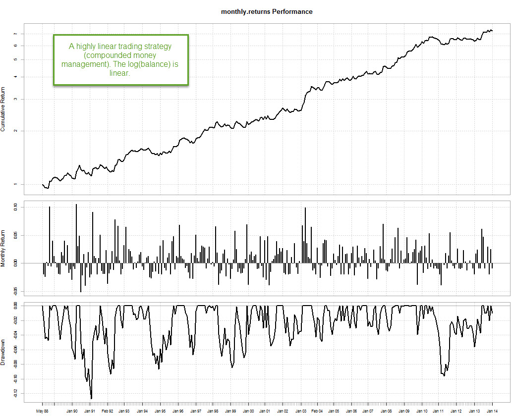
The solution to this problem can be found using the ideal R (IR) statistic. The idea is simply to split the data across a given number of sets containing a smaller portion of our data and then perform separate linear regressions on each case in order to find how the correlation coefficient R^2 changes as a function of time. In this case I am going to split the data in years, but you can also split the data in shorter or larger periods or as a function of trade number instead of time. If you’re system has a trading frequency of more than 10 trades per year you should have no problem in doing a yearly analysis but going lower would clearly be problematic. The ideal R (IR) statistic can then be calculated as the average of the R^2 values found for all sets. The sample strategy showed above seems perfectly linear according to a simple linear regression model, but how will this conclusion change as we calculate the ideal R?

–

resultsTEMP <- read.zoo("C:/pathtocsv/results.csv", 
sep = ",",format="%d/%m/%Y %H:%M", header=TRUE,index.column=1,
colClasses=c("character", "numeric"))

results<- as.xts(resultsTEMP)

resultSplit <- split.xts(results, f="years")

par(mfrow=c(4,6))

correlationCoefficients <- c()

for (i in 1:length(resultSplit) ) {
yearResults <- resultSplit[[i]]
colnames(yearResults)[1] <- "balance"
if (length(yearResults$balance) > 2){
lm.yearResults <- lm(log(balance) ~ index(balance), data= yearResults)

plot(index(yearResults$balance), log(yearResults$balance), 
type="l", main= format(index(yearResults$balance[1]), "%Y"), 
xlab="Date", ylab="log(balance)")

abline(lm(log(yearResults$balance) ~ index(yearResults$balance)))

correlationCoefficients <- c(correlationCoefficients
,summary(lm.yearResults)$r.squared)
}
}

–

–

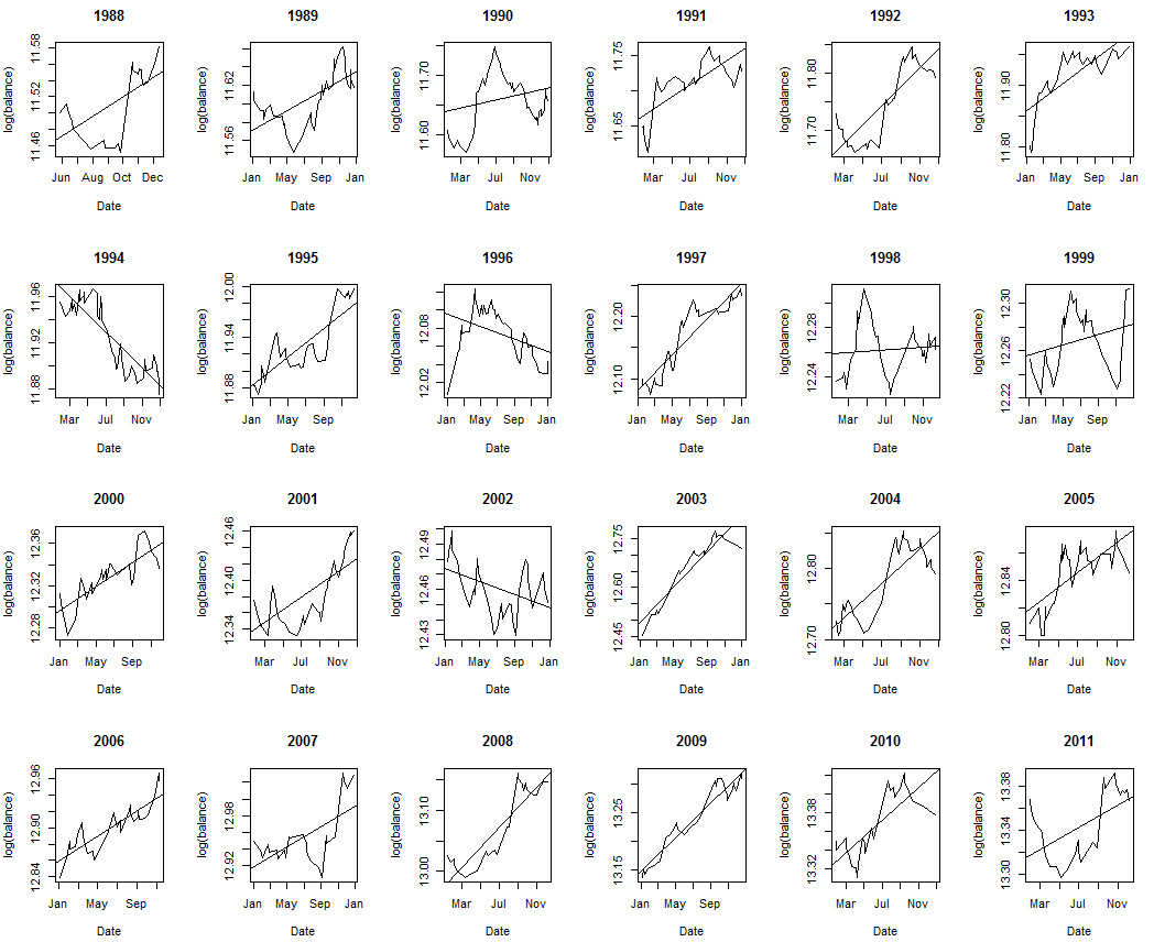
The R code above initially splits the data into yearly periods using the split.xts function, we then calculate linear regressions for every year, save the correlation coefficient within a dataframe and we also plot the linear regression and yearly plots across a 4×6 grid. This allows us to get an overall view of how linear our results are across all the different divisions. Note that the linear regressions and balance plots are made using the log(balance) since the results.csv that I loaded contained compounding returns (therefore we expend the log(balance) Vs time to be linear and not the balance, which would be exponential). The result above shows you that, although the graph looks very linear overall, it suffers from important deviations from linearity when we look at more short term results. The simple linear model gives us an R^2 of 0.98 for this strategy but in reality results are not as smooth as they seem to be from this value. Next we proceed to plot the correlationCoefficients and get the ideal R value.

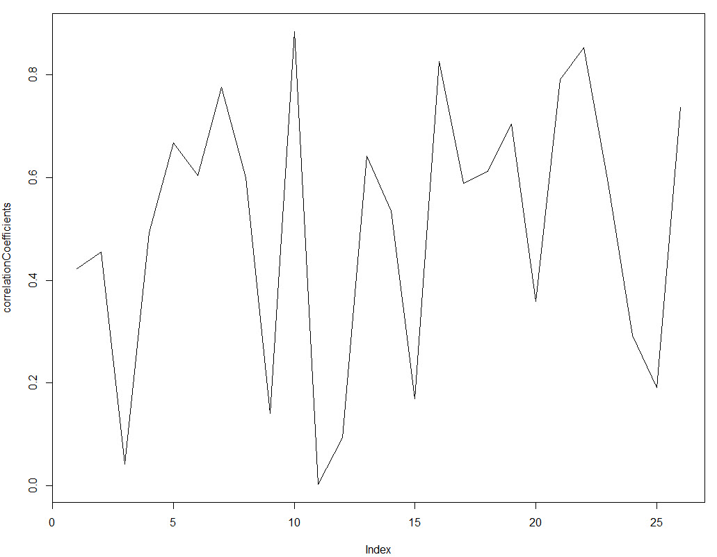
As you can see the correlation coefficients change significantly through time and they very rarely go above the 0.8 mark. The reason is that across short amounts of data a system would need to be extremely linear to get high R^2 values because there is no room for deviations to get compensated over time. You can also see how under some market conditions the correlation coefficient even drops to values close to zero, implying that the strategy – despite its long term linear character – had years where the correlation between balance and time was almost non-existent. The IR value for the strategy is actually 0.50 (average of R squared values over all periods) and the standard deviation of the R squared is 0.26. From these values we can infer that the strategy is still far away from the best possible case  (IR of 1) but since the value is now much smaller it becomes much easier for us to compare different strategies according to their IR results. While the difference between two systems that are highly linear might only be 0.001 of R^2 under a regular simply linear regression of the whole curve, the difference can be as high as 0.1-0.2 when using the IR statistic.

–

par(mfrow=c(1,1))
plot(correlationCoefficients, type="l")

mean(correlationCoefficients)
sd(correlationCoefficients)

–

–

Using the IR statistic you can obtain a performance measurement for your systems that is much more powerful than a simple linear regression. Another advantage is that within its calculation you will get a lot of additional and useful information about your trading strategy (linearity of yearly performance for example). If you would like to learn more about system statistics and how you too can create highly linear trading strategies for your trading  please consider joining Asirikuy.com, a website filled with educational videos, trading systems, development and a sound, honest and transparent approach towards automated trading in general . I hope you enjoyed this article ! :o)