Last week I discussed the use of a simple python script to convert htm based MT4 backtesting results into a format that was easier to analyse by other programs with the aim to perform powerful statistical analysis of our results. On that post we then used R to obtain statistical information for our trading system using the csv file that was extracted from the report by the python script. However despite the fact that R is a really powerful tool for analysis it is clear that expanding the already included libraries can be difficult and some applications – such as embedding of analysis within another program – might be quite difficult. For this reason today I want to talk about how we can also analyse trading system results using the pyfolio library created by the people at quantopian which already contains a large set of system statistics. This library has the advantage of being easily called within python, which allows us to potentially embed analysis within existing applications and easily implement other functionality such as the creation of beautiful statistical analysis reports.
–
#!/usr/bin/env python
#Created by Daniel Fernandez
#http://mechanicalforex.com 2015

import matplotlib.pyplot as plt
import pyfolio as pf
import pandas as pd
import csv
import datetime
import pytz

def lastValue(x):
    try:
        reply = x[-1]
    except:
        reply = None
    return reply

def main():

   tradeTimes = []
   tradeBalance = []

   with open("test.csv", 'rb') as csvfile:
        reader = csv.reader(csvfile)
        i = 0
        for row in reader:
            if i > 0:
                tradeTimes.append(datetime.datetime.strptime(row[0], '%Y.%m.%d %H:%M'))
                tradeBalance.append(float(row[8]))
            i += 1

   returns = pd.Series(data=tradeBalance, index=tradeTimes).resample('D', how=lastValue).pct_change(fill_method='pad').fillna(0).tz_localize('UTC')
–
In order to start our analysis process it is important for you to create a csv file using the python script from last week’s post. Note that you should also have the pandas and pyfolio libraries installed into your system (latest python versions can get this done with a simple “pip install pyfolio” command). After you install the libraries and generate the csv (change the “test.csv” in the script to point to the path of our csv) you can then use the above script to load the results into a pandas time series object which will allow us to use the pyfolio library to perform analysis. The time series contains the daily return information from the strategy which has been obtained from the balance/time information and refactored to the daily timeframe. Note that the time series has been localized to UTC (even if your back-testing data is in another TZ you should have UTC as the final localization TZ) this due to the fact that the pyfolio library will generate an error if a time series either misses localization or is localized to something other than UTC. If your time series is in a different TZ you can first localize to that timezone and then convert to UTC.
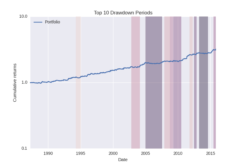
Once we have our pandas time series loaded we can then perform a series of actions using the pyfolio library in order to obtain statistical analysis information. One of the most useful pieces of information that we can obtain is a plot of the drawdown periods coupled with an “underwater plot” that shows us both the top 10 drawdown periods of our strategy plus the drawdown behavior throughout the backtest. The code below generates these two plots. Note how I have changed the Y axis of the plot that highlights the drawdown periods to logarithmic, in this manner we will be able to visualize heavily compounded plots without the visual distortions caused by the compounding effect (which makes losses at a later stage in a back-test appear bigger when they might be much smaller than losses in the beginning).
–
    fig = plt.figure(facecolor='white')
    plt.yscale('log')
    ax = pf.plot_drawdown_periods(returns).set_xlabel('Date')
    plt.savefig('drawdownPeriods.png')

    fig = plt.figure(facecolor='white')
    ax = pf.plot_drawdown_underwater(returns)
    plt.savefig('underwaterPlot.png')
–
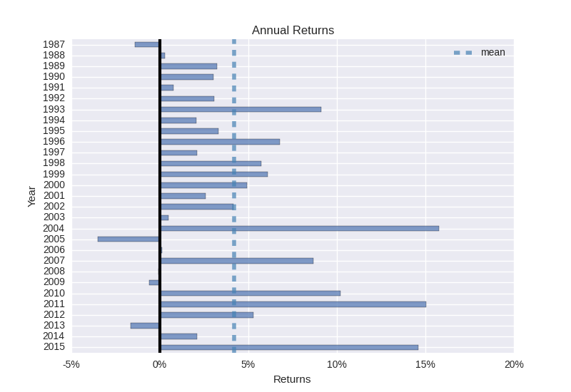
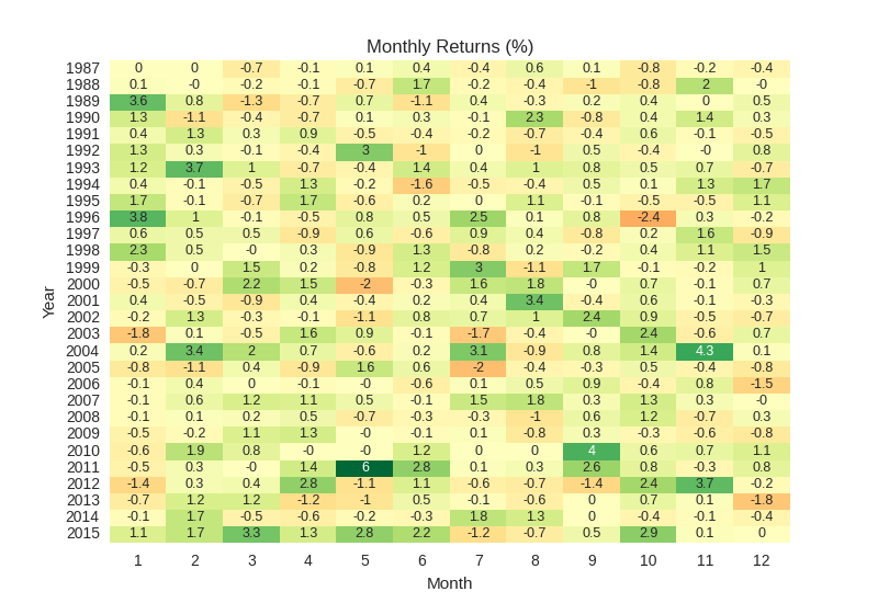
Two other plots that I consider very useful for system analysis have to do with the annual and monthly return distributions of your system. These are useful in order to know how disperse your distributions of longer term returns are and for example how likely you are to experience a losing month/year and how low and high are your best and worst performing periods. The pyfolio library has some very handy plots for the display of this information that you can obtain using the code below. I particularly like their implementation of the monthly heatmap since it shows you in a single graph the results you have had for every month plus your best and worst months. A quick glance at this plot can already tell you if you have had particularly good or bad years and how well distributed your monthly returns are.
–
    fig = plt.figure(facecolor='white')
    ax = pf.plot_monthly_returns_heatmap(returns)
    plt.savefig('monthlyReturns.png')

    fig = plt.figure(facecolor='white')
    ax = pf.plot_annual_returns(returns)
    plt.savefig('annualReturns.png')
–
The above are just two quick examples of what you can obtain with the pyfolio library but you should definitely check out the plotting section of their code to learn more about the functions that are available for the creation of other useful plots. Many additional useful plots such as the rolling returns and frequency distribution of monthly returns are possible with the pyfolio library. The calculation of standalone statistics is also very easy to carry out, you can obtain information by simply calling functions from the timeseries section of their library. As an example you can print the maximum drawdown in the above code by simply issuing the “print pf.max_drawdown(returns)” command, or the Sharpe ratio by using the “print pf.sharpe_ratio(returns)” directive.
In summary the pyfolio library provides you with a powerful tool to perform statistical analysis of your MT4 trading results (or any other results that you can put into a pandas time series). The pyfolio library has the advantage that it’s code is easier to expand and modify and that you can directly call it within python. With pyfolio you can potentially create beautiful statistical analysis reports for your strategy (which could even be performed on batches of report files using a script) or you can even use the calculation of statistical data like the Sharpe ratio for a portfolio optimization or analysis script (which we will do on a future post!).
If you want to learn more about my work in automated trading and how you too can learn to create and use your own portfolio of algorithmic trading strategies please consider joining Asirikuy.com, a website filled with educational videos, trading systems, development and a sound, honest and transparent approach towards automated trading.


