On a recent post I discussed the creation of an RSI based neural network algorithm using RSI indicator values as inputs. These algorithms were able to achieve good results on the EUR/USD and were primarily based on using RSI indicator values from two predetermined periods and different shifts as inputs for the construction of the examples used to constantly retrain the neural network. Despite the success of these algorithms I wondered what would happen if the RSI inputs were simplified (use one period instead of two) and what would happen if the period of the RSI values was changed. On today’s post I am going to discuss my results using single period RSI algorithms as well as the effects that period changes and training changes have on the performance of the systems.
–
//code modifications in the regression_i_simpleReturn_o_tradeOutcome function

for(j=0;j<barsUsed;j++){
       inputs.element(m)[j] = iRSI(0,indicatorPeriod,tl+j+i+1)/100;
        }

//code modifications in the p_regression_i_simpleReturn function


for (j=0;j<barsUsed;j++){
         inputs.element(0)[j] = iRSI(0,indicatorPeriod,j+1)/100;
		}
–
The algorithm setup is identical to that of my previous post on an RSI machine learning system except for the fact that the input/output building functions have been changed according to the above code. Instead of having two fixed period values for the construction of inputs we now have half the inputs and only one indicator period used for construction. Asirikuy members can modify the above mentioned functions to reproduce my results. Note that the indicatorPeriod function parameter needs to be added to the functions and header files as well as to the function and header files of the NN_Prediction_i_simpleReturn_o_simpleReturn function in the Asirikuy Machine Learning library in F4. You should also add this indicatorPeriod as an external parameter to the trading system used so that you can assign it different values. In the system I will be discussing today the NN is retrained (300 epochs) before every trade using the last 140 examples, each one built with 4 RSI indicator values as inputs and the trade outcome variables explained in the last post as outputs. The system trades only at 0 GMT +1/+2.
–
–
The first thing I noticed with this single period RSI algorithms was that finding profitable systems had the same difficulty as when using two indicator periods. Systems found with two different groups of RSI inputs had similar linearity and compounding efficiency characteristics with systems also having rather similar risk adjusted returns. Maximum drawdown values as well as CAGR statistics were very similar between both system types with none of them drawing a clear advantage over the other. However the greater simplicity of the single indicator group implies smaller potential for data-mining bias so overall this approach seems to be better than the one discussed on my previous post.
An interesting experiment is to vary the RSI period for the inputs to see how sensitive the system actually is to this parameter. Overall the system turns out to be quite robust to significant changes in the RSI with only moves towards very low (10) or very high (50) periods causing significant deviation in terms of profitability. The best RSI value for this setup turned out to be a period of 36, but systems produced with variations from 32 to 40 turn out to be quite similar as you can see on the graph above. It is interesting to also note how performance is rather similar for all algorithms up to around 2007, after this point there is a significant divergence in model results with the 32-40 period group becoming the only one successful, all other things being equal. It is also worth noting that all algorithms give positive 28 year results, highlighting the predictive power of the RSI despite the variations in parameter values.
–
–
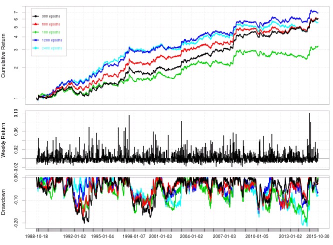
Another interesting point is to consider the number of training epochs used for the above experiments. It may well be that 300 epochs (the low value I used to make the experiment more computationally feasible) is not high enough to provide the best possible results for this algorithm. Further increases in the number of training epochs for the neural network can appear to improve results (as showed in the graph above) but actually the Sharpe ratio increases substantially from using 100 epochs (0.86) to 300 epochs (1.26) and then ceases to increase substantially with 600 epochs (1.21), 1200 epochs (1.26) and 2400 epochs (1.20). As risk adjusted returns remain fairly constant around a value of 1.22 after 300 epochs we might consider that the algorithms are already well trained at this point for the entire price series, particularly for this RSI period values. It is also important to note how these large increases in epochs above 300 do not lead to important drops in the Sharpe ratio meaning that this inputs have some robustness towards over-fitting under these conditions.
The above RSI neural network based algorithms which use single indicator values and are particularly well trained at low numbers of epochs (300) are a computationally feasible route for the intensive mining of machine learning algorithms since at this cost evaluating DMB is feasible. Further exploration of different RSI configurations and network topologies might provide further enhancements while results on different trading symbols and timeframes will also speak about the robustness of these neural networks. If you would like to learn more about the building of constantly retrained machine learning strategies please consider joining Asirikuy.com, a website filled with educational videos, trading systems, development and a sound, honest and transparent approach towards automated trading.


