If you have ever read my blog you may already be aware of how important correlations are when designing algorithmic trading portfolios. Knowing how all strategies relate is vital since this will tend to determine the level of diversification within a trading setup. Generally we perform correlation measurements by calculating a correlations between the return series of two different trading strategies but today I want to take this a step further with a measurement I have devised called the “rolling correlation index”. Today I am going to introduce this index and talk about why it is such a powerful tool for the evaluation of system correlations when compared with something much simpler, such as the all-time pearson correlation coefficient of the return series. I will also go through a python example showing you how to obtain the values for the index, including sample data so that you can reproduce and play with the values showed within this post. You can download a zip containing the script and data here.
–
#!/usr/bin/python
#Programmed by Daniel Fernandez
#http://mechanicalforex.com
#https://asirikuy.com
#Follow me on twitter @asirikuy

import subprocess
import sys
import linecache
from tempfile import mkstemp
from shutil import copy
from os import remove
from os import rename
from datetime import datetime
import argparse
import pandas as pd
import csv
import os
import re

def lastValue(x):
    try:
        reply = x[-1]
    except:
        reply = None
    return reply

def tryint(s):
    try:
        return int(s)
    except:
        return s

def alphanum_key(s):
    """ Turn a string into a list of string and number chunks.
        "z23a" -> ["z", 23, "a"]
    """
    return [ tryint(c) for c in re.split('([0-9]+)', s) ]

def sort_nicely(l):
    """ Sort the given list in the way that humans expect.
    """
    l.sort(key=alphanum_key)

def main():

    indir = './bcktest'
    backtestFileList = []
    backtestFiles = ""
    for root, dirs, filenames in os.walk(indir):
        for f in filenames:
            if "sys" in f:
                backtestFileList.append("bcktest/" + f)

    sort_nicely(backtestFileList)

    j = 0

    for item in backtestFileList:

        print item

        tradeTimes = []
        tradeBalance = []

        with open(item, 'rb') as csvfile:
            reader = csv.reader(csvfile)
            i = 0
            for row in reader:
                if i > 0:
                    tradeTimes.append(datetime.strptime(row[3], '%d/%m/%Y %H:%M'))
                    tradeBalance.append(float(row[10]))
                i += 1

        if j == 0:
            allTimeSeries = pd.Series(data=tradeBalance, index=tradeTimes).resample('M', how=lastValue).pct_change(fill_method='pad').fillna(0)
        else:
            allTimeSeries = pd.concat([allTimeSeries, pd.Series(data=tradeBalance, index=tradeTimes).resample('M', how=lastValue).pct_change(fill_method='pad').fillna(0)], axis=1)


        j += 1

    allTimeSeries = allTimeSeries.fillna(0)

    all_RCI = []

    for i in range(len(allTimeSeries.columns)):

        RCI_values = []
        returns1 = allTimeSeries.iloc[:,i]

        for j in range(len(allTimeSeries.columns)):
            returns2 = allTimeSeries.iloc[:,j]
            if i != j:
                rolling_correlations = pd.rolling_corr(arg1=returns1, arg2=returns2, window=6).dropna()
                RCI = (rolling_correlations > 0.5).sum()
                print "index is {}".format(RCI)
                RCI_values.append(RCI)
            else:
                RCI_values.append(0.0)

        all_RCI.append(RCI_values)


    correlations = pd.DataFrame(all_RCI)

    import matplotlib.pyplot as plt
    fig, ax = plt.subplots(figsize=(12,9), dpi=100)
    heatmap = ax.matshow(correlations, aspect = 'auto', origin = 'lower', cmap ="RdYlBu")

    ax.invert_yaxis()
    ax.xaxis.tick_top()

    plt.show()


##################################
###           MAIN           ####
##################################

if __name__ == "__main__": main()
–
When we want to know how different two systems really are and how much diversifying power there is to trading them together we resort to correlation measurements. In general systems that have highly correlated returns will tend to magnify drawdowns and profit cycles – increase overall volatility – but systems that have low correlations will tend to smooth the equity curve due to the hedging of each others drawdown cycles. We tend to evaluate correlations using the pearson correlation coefficient (R) which is nothing more than a number representing how linear the relationship between the returns of two systems are or more precisely how small the residuals from a linear regression line between both return series are. The pearson correlation coefficient can have a maximum value of 1 and a minimum value of -1 with 1 meaning perfectly correlated and -1 meaning perfectly inverse (perfect opposite) and 0 meaning no correlation at all.
The main problem with the pearson correlation coefficient is that it provides us with a global measurement that encompasses the entire return series but says nothing about fat-tail events that cause correlations between strategies to go higher in the short term. We are generally not especially worried about maintaining a low correlation after 30 years of trading but we’re generally worried about how things correlate under short term circumstances. We are mostly worried about two systems joining forces to deepen a drawdown within a 6-12 months period even if their overall correlation after and before that event is 0. While a very strong short term correlation will have a very profound effect in terms of performance – can deepen a max drawdown event – it will have little effect in terms of the longer term pearson correlation coefficient.
–

–
For this reason I have decided to come up with a measurement that better reflects what we want to do when we talk about systems being uncorrelated. The Rolling Correlation Index (RCI) sums up the occurrence of short term, high correlation events that greatly detract from the diversification power of two trading strategies. It is obtained by calculating the rolling correlation of returns for the past 6 months between two monthly return series and then adding 1 for each time the correlation value exceeds the 0.5 threshold. Overall this means that two strategies can be largely uncorrelated most of the time but can still have a high RCI value if they just happen to become correlated when uncorrelated behavior is needed the most.
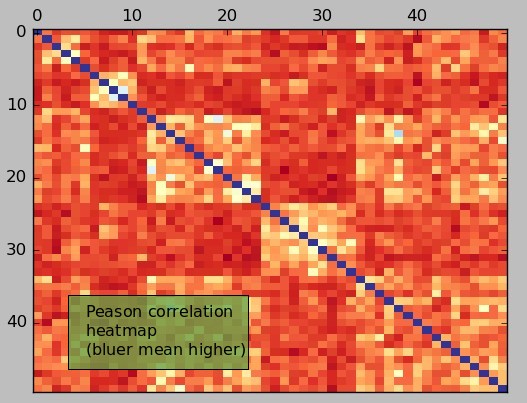
The above python script calculates the RCI value for a group of 50 price action based systems that have been back-tested for the past 29 years. The first image above is the R heatmap showing the pearson correlation coefficients between the 50 systems. As you can see all systems have a low overall correlation (R<0.5), There are “blocks” of systems which are closer to this 0.5 value between them mostly because they come from similar mining spaces or because they come from the same trading symbol. As you can see the pearson correlation analysis says nothing about the short term correlation but gives us a broad and wide view of how correlated the strategies are.
–

–
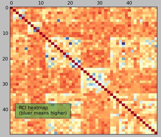
The RCI correlation heatmap – second image above – is a different story. Of course the overall correlations are similar between the systems – after all they have low long term correlations – but we can see that there are several systems that have a substantially higher RCI value while they have a relatively low R. There are now some evident “dark blue” dots within the entire heatmap showing that there are indeed some systems that tend to correlate much more than the average repository under the short term. The mean of the RCI is 69.76 while the highest values are in the order of 180 to 220. This means that there are on average 69 periods where the 6 month rolling correlation has an R higher than 0.5 while in the upper side we have cases where this value is in the order of 180 to 220 days. On the lower side the systems with the lowest RCI values have magnitudes in the order of 20-40. In general you could obtain a much more tightly woven portfolio with less historical short term correlation if you chose to use an RCI filter of 60 than if you used an R lower than 0.5.
Of course the biggest question is whether the RCI value is of any predictive value. Is having a low RCI predictive of systems that will retain low rolling correlations or are rolling correlations a matter of chance and filtering systems by RCI is worthless in practice? I will monitor our system repository to get a better idea of how RCI values change with time to see if the frequency distribution of RCI values within our portfolios changes as a function of time. If you would like to learn more about correlation analysis and how you too can learn how to use large portfolios using thousands of uncorrelated strategies please consider joining Asirikuy.com, a website filled with educational videos, trading systems, development and a sound, honest and transparent approach towards automated trading.


