Mechanical Forex

Once every few years a very novel way to look at things comes to light. This is what happened in 2014 when Abbas Golestani and Robin Gras published their time series forecasting paper on Nature scientific reports. In this paper they expose a new methodology for the prediction of time series which seems to almost miraculously predict some extremely difficult to solve problems in several areas, including financial time series. The paper shows some impressing predictions on the DJIA that pretty much destroy predictions using ARIMA and GARCH models. Soon after this paper was released I reproduced some of the their results but faced several issues that prevented me from really using this method up until now. Within this series of blog posts I want to show you how you can reproduce this prediction method using R and what the problems of using it might be. I will walk you through the ideas behind the methodology and the problems it faces for practical applications.

–

library(quantmod)
library(fractaldim)

#Programmed by Dr. Daniel Fernandez 2014-2016
#https://Asirikuy.com
#http://MechanicalForex.com

getSymbols("SPY",src="yahoo", from="1990-01-01")

# We want to predict the SPY after index 2000
endingIndex <- 2000
SPY_TEST <- SPY$SPY.Adjusted[1:endingIndex]

#These are the fractal dimension calculation parameters
#see the fractaldim library reference for more info

method <- "rodogram"

#number of samples to draw for each guess
random_sample_count <- 50

Sm <- as.data.frame(SPY_TEST, row.names = NULL)

#do 500 predictions of next values in Sm
for(i in 1:500){
  
  delta <- c()
  
  # calculate delta between consecutive Sm values to use for the 
  # building of the normal distribution to draw guesses
  for(j in 2:length(Sm$SPY.Adjusted)){
    delta <- rbind(delta, Sm$SPY.Adjusted[j]-Sm$SPY.Adjusted[j-1])
  }
  
  # calculate standard deviation of delta
  Std_delta <- apply(delta, 2, sd)
  
  #update fractal dimension used as reference
  V_Reference <- fd.estimate(Sm$SPY.Adjusted, method=method, trim=TRUE)$fd
 
  # create N guesses drawing from the normal distribution
  # use the last value of Sm as mean and the standard deviation
  # of delta as the deviation
  Sm_guesses <- rnorm(random_sample_count , mean=Sm$SPY.Adjusted[length(Sm$SPY.Adjusted)], sd=Std_delta )
  
  minDifference = 1000000
  
  # check the fractal dimension of Sm plus each different guess and
  # choose the value with the least difference with the reference
  for(j in 1:length(Sm_guesses)){
    new_Sm <- rbind(Sm, Sm_guesses[j])
    new_V_Reference <- fd.estimate(new_Sm$SPY.Adjusted, method=method, trim=TRUE)$fd
    
    if (abs(new_V_Reference - V_Reference) < minDifference ){      
      Sm_prediction <- Sm_guesses[j]
      minDifference = abs(new_V_Reference - V_Reference)
    }
  }
  
  print(i)
  #add prediction to Sm
  Sm <- rbind(Sm, Sm_prediction)
}

plot(Sm$SPY.Adjusted, type="l", xlab="Value Index", ylab="Adjusted Close", main="SPY Rodogram")
lines(as.data.frame(SPY$SPY.Adjusted[1:(endingIndex+500)], row.names = NULL), col="blue")

–

The main idea behind the entire paper is actually quite simple and has a very interesting assumption at its core. The paper tells us that time series such as financial time series are chaotic and therefore their chaos related properties should remain constant as a function of time. If you can think about possible future values for a time series then the most reasonable future value is the one that best preserves the underlying chaos related properties of the series. Therefore if you can think about a chaos related property this property should remain constant and therefore anything you add should provide the least possible variation from this value when the property is measured again.

The practical way to do this is quite simple as well. Golestani and Gras suggest the use of the Lyapunov exponent or fractal dimension as chaos series properties and propose a simple methodology for forecasting. First calculate your chaos property for the entire series, then create a distribution that represents the variation between elements of the series and make random draws from this distribution such that you can have candidates for the next value of the series, then recalculate your chaos property again after adding each candidate and choose the new series that has the value closest to the original reference value of the property. In essence you simply gather many potential guesses and add whichever perturbs the chaos property the least.

–

–

The actual real implementation is a bit more complicated because both the Lyapunov exponent and the fractal dimension are really not “formally defined”. When you calculate the Lyapunov exponent you usually have 8 parameters to choose from and there is virtually no formal way to choose most of these parameters. Parameters like the number of points to take into account are simply not intuitively assignable. The fractal dimension poses a similar problem, there are more than 5 different methods for the calculation of the fractal dimension of a financial time series, with more than 8 implemented in the R fractaldim library, posing a similar problem to the Lyapunov exponent calculation. I think you can start to see how this creates a very important issue when dealing with time series predictions.

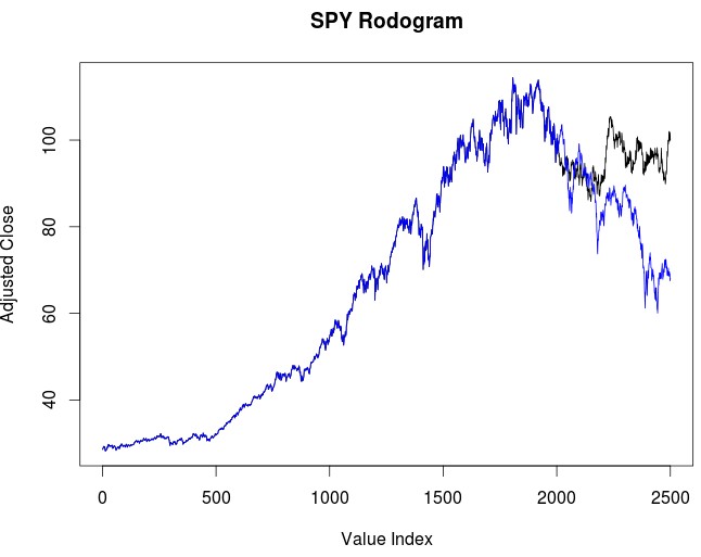
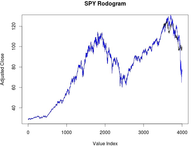
In the end I decided to go with the fractal dimension implementation as it poses a far less daunting problem since in the end it comes down to a choice of method for calculation instead of having to iterate through billions of potential parameter combinations. The implementation you see above in R can be used to predict 500 daily return SPY values right next to the 1999 bubble, where the SPY lost a very significant portion of its value (you can change the endingIndex value to change the period, the 2008 crisis is around 3500). Before this point the time series had basically no significant down trending component (from 1990 to 2000) and therefore this poses a very interesting problem for time series prediction. If this works the method basically has to predict that the SPY has to drop even if there is no precedent for such a drop within the data. Basically all machine learning and technical analysis methods would fail to forecast such a drop since it is simply outside of the historical scope. But can the chaos predictions fare better?

–

–

As you can see in the first image within the post the prediction using rodogram calculated fractal dimension values fails to properly account for the drop during the dotcom bubble, although the prediction is quite accurate during the first 200 days there is a dramatic difference in the ending result due to the method completely missing the biggest portion of the drop and heavily underestimating a recovery. Of course this is still far better than what any ARIMA forecast could tell you for a 500 day horizon but it is still not a very good long term forecast.  We can also see what happens when we go to the 2008 crisis to see if the method actually fares better with more data. It may well be possible that we needed to include a crisis period within the data before the fractal dimension accurately converged to its “long term value”. If the method is based on the notion that the fractal dimension does not change then it is reasonable to conclude that prediction accuracy should increase with larger data sets.

I was not disappointed with the forecasting results for the 2008-2009 period using the Rodogram calculated fractal dimension (second image within the post), not only does the forecasting method reproduce the double top in the SPY but it also reproduced the move from a practically vertical bull market to a very steep bear market. This shows us that the more data we add the more accurate the results of the algorithm become. This is by far the only method I know of that can produce such an accurate 500 day forecast, especially within such a significant market shift.

Of course there are many things yet to explore using this method. Does it fare well in currencies? Does it work on other instruments? What happens when you use other fractal dimension calculation methods? Does it work better at certain prediction horizons? What is the probability to obtain a good forecast just by chance? The answers to all of these questions will come on future blog posts. If you would like to learn more about financial time series and how you to can learn to create systems to trade them  please consider joining Asirikuy.com, a website filled with educational videos, trading systems, development and a sound, honest and transparent approach towards automated trading.