Mechanical Forex

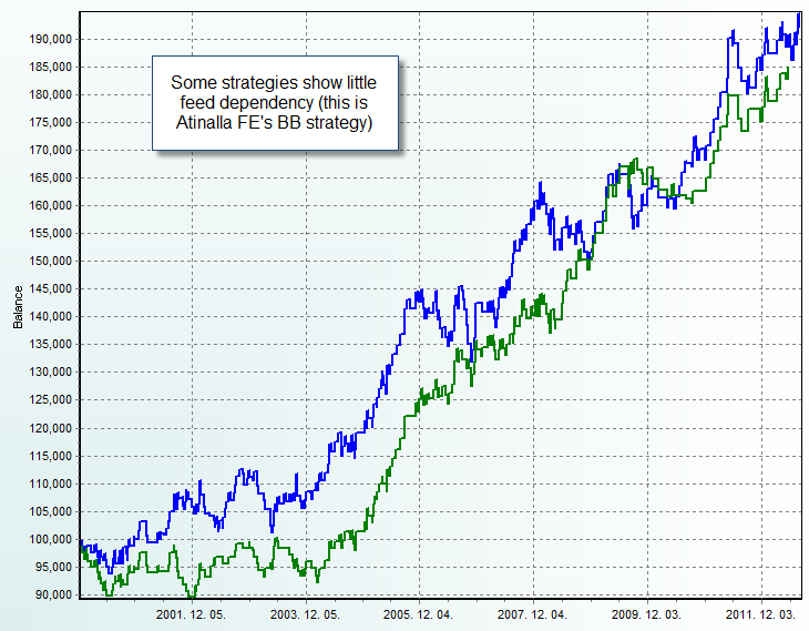
Perhaps one of the worst things about the Forex market is that there is no central exchange to trade but a conglomerate of financial institutions that allows the exchanging of foreign currencies through a rather disorganized network where no unique well rounded order book exists. The problem this brings us is that when designing algorithmic strategies we have to consider the effect that feed variations may have since we know our historical data is not going to be the “only feed” but a rather “possible feed” from the hundreds that may in the end be available (if you count retail broker smoothing, liquidity provider combinations, etc). The problem of testing feed variations is also that you need to find at least two different feeds that were equally plausibly tradeable in the past as you cannot simply distort a feed for a realistic comparison.

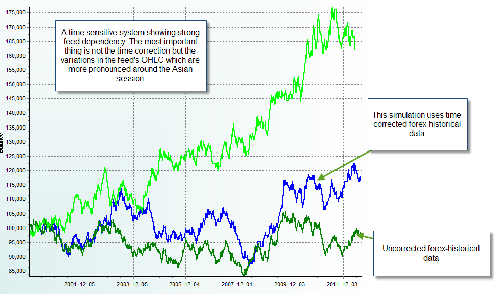
Previously in Asirikuy we only had an Alpari UK 12 year historic feed (with nothing to compare it to) but recently we have had access to a 25 year old data set from forex-historical which allows us to do a direct comparison between results drawn from Alpari UK and those drawn from the forex-historical data. Since we didn’t log the data ourselves – we get them from the providers – we have to assume that both data sets are equally valid and test our systems as if they were facing two different brokers. Thanks to F4’s ability to normalize different historical data sets to match the exact same time shift – even if they are on different ones – we now have the ability to even compare time sensitive strategies (something we hadn’t been able to do before). Through this post I want to start the discussion about differences between systems, talking about the causes and effects of these – sometimes large – differences. This will certainly lead to better design rules for systems and to better decisions in choosing systems for live trading.

–

–

Let me start by saying that there is no clear obvious “one rule” or characteristic that bundles all strategies that show feed dependency (very different results between two data feeds). For example I initially had a suspicion that only time-sensitive systems (those that filter hours somehow) were more prone to dependency than others but this was clearly not the case as some systems that do not use time filtering also showed this type of results and some time filtered systems were also very well-behaved. The issues is therefore not related specifically to time filtering but to other much more fundamental characteristics of a trading strategy. Trade number was also something I thought could be influential – as more frequently trading strategies could perhaps be less dependent – but some instances with very high trade numbers also showed significant dependency measurements.

So in order to understand what causes feed dependency I needed to look into the kernel of the issue. What makes a system trade very similarly in two cases while another trades very differently in another case? The answer seems to be related with the sensitivity of a system’s entry singling mechanism. Let us suppose that a system takes signals based on a single oscillator crossing event but this only happens if an oscillator moves in a very specific way (crosses down from X then up to Y then down to Z) let us suppose that Y and Z can also be the same such that the  system simply trades when there is a cross down from X. These are two cases of the same system, the first – in my experience – is prone to very high feed dependency while the second is not. The reason is that there are many possible variations that may lead to the same entry in the second case while the first case is very specific and can easily curve-fit to a particular data feed.

–

–

Many of you may be thinking – aha – degrees of freedom, but the case isn’t this simple because a strategy can have many degrees of freedom in theory and still give very small dependency provided that those degrees of freedom aren’t fully expressed in the actual entry logic used. This case is showed in the example above. This is why for some Asirikuy systems there is big feed dependency on some instances of a system while for another there is almost none. The main difference is that on one of them the degrees of freedom are not fully expressed – the strategy is more generalized – while on another degrees of freedom are excessively expressed (the strategy is very curve-fitted). It should also be considered that sometimes degrees of freedom aren’t as obvious as they appear because different variables might be implicitly correlated. Some systems with very large degrees of freedom can therefore give good results because their logic inherently correlates this degrees of freedom and makes their effect less pronounced.

The problem then could easily be solved by restraining degrees of freedom? Not entirely. Some systems show feed dependency due to problems dealing with constraints. Very specific time constraints – especially those that allow trading only during a particular single hour – may make the system exceedingly dependent on some particular portion of the data feed which might be more variable between feeds than the other. For example a system that trades immediately after the Asian session suffers from a problem dealing with data feed differences on this period which are more pronounced than on other trading sessions. Therefore this system has a lower chance of not being feed dependent – even if its degrees of freedom are scarce – because of the simple nature of the trading strategy.

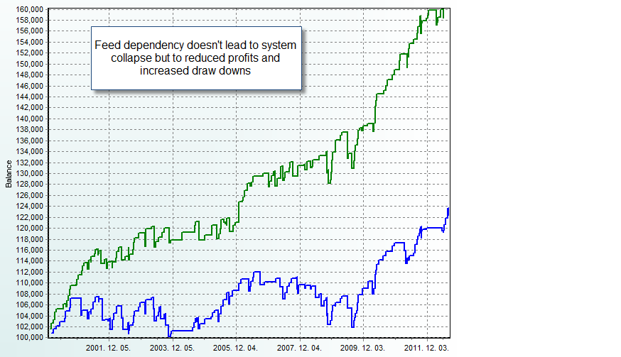
However an interesting effect is that although systems that show feed dependency generally lose a significant portion of their trading edge, none become disastrous. This means that although they have much lower AAR to DD ratios, none of the actually goes into and end-less spiral that kills the account. In all pronounced cases I have examined the systems go from a profitable to a break-even state along the testing period. This means that the price of trading a feed dependent system – on a feed that doesn’t match the reference feed very well from a candle OHLC perspective – is that the system will simply not be profitable but probably it will not wreck havoc.

–

–

In practice however it is clear that systems that show limited feed dependency are more desirable – naturally less curve fitted – and therefore these should be used for live trading purposes rather than feed dependent systems (from a robustness point of view). Right now we are building a full F4 system DB using ADA which will allow us to compare Forex-historical and Alpari UK back-tests to determine which Asirikuy systems are most affected and which ones are affected the least. I will also be writing some more blog posts about this matter within the next few days and weeks so stay tuned for more analysis and information :o).

If you would like to learn more about system analysis and how you can better understand your trading strategies  please consider joining Asirikuy.com, a website filled with educational videos, trading systems, development and a sound, honest and transparent approach towards automated trading in general . I hope you enjoyed this article ! :o)