Mechanical Forex

If you have been reading my blog during the past year you may have noticed many posts describing all sorts of different input/output structures for the creation of constantly retraining machine learning systems for trading the Forex markets. Whenever I post one of these structures I generally mention that it is capable of generating highly stable systems through long term historical tests and that it can therefore lead to usable setups. Nonetheless – given the amount of potential input/output structures – it is very important to consider how we can compare one set of machine learning I/O with another. On today’s post I am going to talk about how to establish a solid methodology to make these comparisons possible. Additionally I will also talk about why the general methodologies used in academic machine learning are really not useful for this specific problem.

–

–

In traditional machine learning judging the quality of an input structure against another is not considered a difficult task. You have a given set of predictions that you want to make and you have a model that trains based on past examples of these predictions – your outputs – that you can use on a set that is outside of the machine learning’s training set to judge the accuracy of the model and the usability of the input structures. If you are making a model to detect cat faces and you want to compare two different input types the process is relatively straightforward. Take a set that contains cat faces and non-cat faces then train both models on it and see which one is more accurate on a new set containing a new set of pictures. If the first set of inputs gives 60% correct predictions and the second 80% then you’re all set, the second set of inputs is definitely better.

In trading things are far more complicated. The main reason for this is that we do not care about accuracy in predicting outputs – this is why the title of this post contains input/output instead of just input – but we care only about the statistical properties of the resulting trading systems. If making decisions based on using past daily returns as inputs and the next day’s directionality as output can yield predictions that create systems with good statistical properties (good Sharpe, R², etc) we really do not care if there we only make good predictions 20% of the time. In trading you can have incredibly good systems even if you have low accuracy in your outputs because what matters is the distribution of those predictions. For example if you’re predicting the next day’s directionality you can be profitable if you predict the days with the largest returns and fail on most other days. If you focus on your accuracy in output prediction you will fail to get better systems, which is really our end goal. As mentioned on most of my previous posts constant retraining of the models is also key to achieve profitable machine learning models.

–

–

Given that we need to evaluate if an input/output structure is better than another in terms of the system results they generate then things seem manageable. Simply get a system back-test using both structures and choose the one with better statistics. Nonetheless the problem is far more complicated because each input/output structure can generate more than 1 system given that they are parametric in nature. For example if you choose to use past bar returns as inputs then how many bars you use to build each example and how many examples you use for the moving window used for retraining can affect the results of the algorithms. Perhaps an input/output structure generates great systems with a 20 example moving window and another structure requires 200. Which is better?

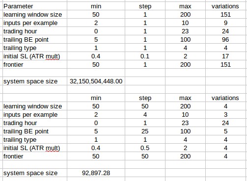
To address this we would then need to consider the total possible number of systems that can be generated and compare the distributions of trading statistics for both cases. In the case of the past bar return/ trade outcome algorithms we use  – see my past blog posts for more information about this – this number can become really big, really quickly because of the number of possible parameters present within the input/output structure. If you see the first image above you’ll see that given the finest variations in the parameters we use we would expect to have something like 32 billion possible systems. Evaluating this is simply unfeasible and we therefore need to simplify the problem to something that is tractable.

–

–

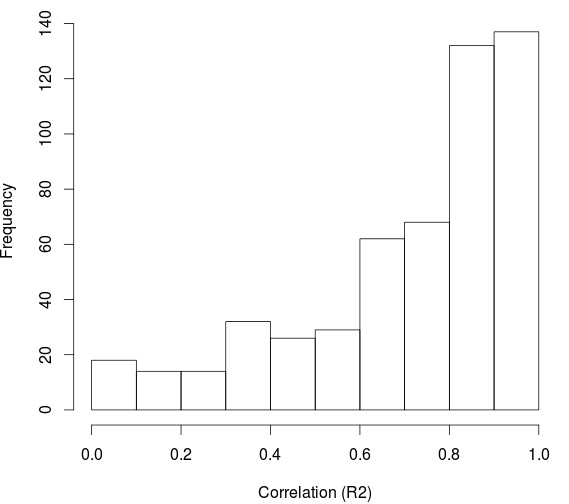
To obtain a good image of what the system space statistics look like we really don’t need the 32 billion systems. Given the fact that we expect neighboring parameters to be highly correlated for most parameter variations – as shown in the second graph above – we can then reduce the parameter space by making variations in parameters where neighboring correlations are expected to be high coarser. In the first graph above you can see the reduction we can carry out by making most parameters much coarser. Of course some parameters violate the neighboring correlation assumption – like the trading hour and the trailing stop type – reason why the number of variations for these parameters cannot be reduced.

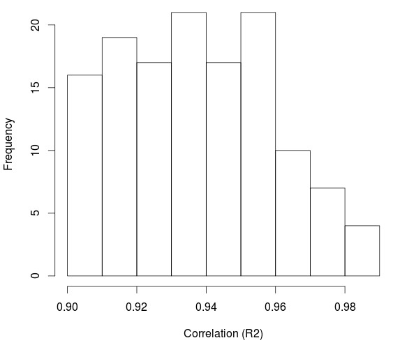
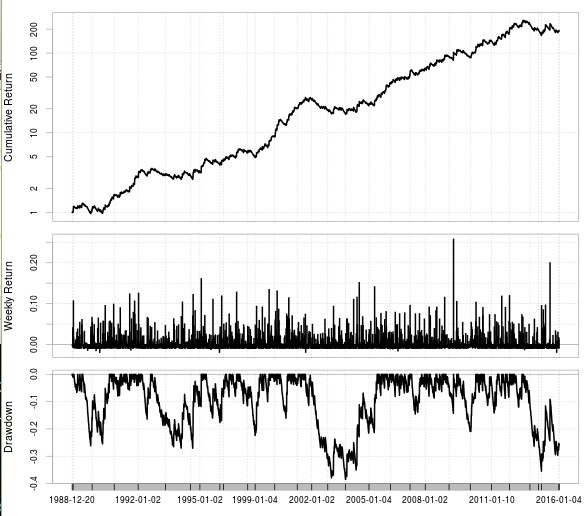
With this we now get 92,897 iterations which is something that – although still quite big – can be evaluated significantly well. Additionally we can employ another trick to make things even easier for us. We do not really need to sample the 92,897 possibilities but we can in fact only sample as many as we need to obtain a distribution of system statistics that does not vary significantly. If you sample systems from the available space until the distribution of the statistic you want to evaluate converges you can then get away with only testing around 2000-3000 tests (which we can do in under a day). In the third image above I show you the distribution of the R² statistic for a machine learning input/output structure. First we have the distribution of R² excluding only unprofitable systems and systems with low frequency (less than 10 trades per year) and in the second distribution we have the R² > 0.9 distribution. Below a sample system with R² = 0.98 found on the coarse grid.

–

–

Given that we only care for highly linear systems we can easily establish a benchmark by calculating the percentage of systems that have an R² > 0.9 from the number of tested samples. In this sample case that would be (140/2691)*100 which would be 5.20%. We now know that for this input/output structure we have an expectation that around 5.2% of the space will generate high quality strategies. This value can be compared with values from other input/output structures to decide which one might be better than another. If here we have 5% and in another we have 20% then obviously the 20% one would be better. I would also like to point out that it does not make sense to use much more astringent filters here (like for example Sharpe > X or R² > 0.99) because our grid is too coarse. Although when performing the final DMB analysis of slices of this space we can be much more picky for the initial input/output comparisons on extremely coarse parameter grids this makes little sense.

If you would like to learn more about how to create constantly retraining machine learning systems to trade the Forex market please consider joining Asirikuy.com, a website filled with educational videos, trading systems, development and a sound, honest and transparent approach towards automated trading in general.