Mechanical Forex

A couple of months ago I wrote a post about system performance and how the worst case statistic expectations for our strategies can change depending on the trading horizon we’re confronting. On that post I gave some basic code to be able to draw distributions using python and we saw how the distribution of Sharpe ratios for a short and long trading scenario could vary very significantly. On today’s post I am going to show you how you can track the evolution of a couple of worst case statistics as a function of trading time using the qq-pat library, an open source financial time series analysis library programmed by Jorge Ferrando and myself. I will be showing some sample code using an Asirikuy price action based trading strategy and we’ll discuss how the worst case statistics evolve through time.

–

import pandas as pd
import datetime
import qqpat
import csv

def lastValue(x):
    try:
        reply = x[-1]
    except:
        reply = None
    return reply

tradeTimes = []
tradeBalance = []

with open("sample_system_test.txt", 'rb') as csvfile:
        reader = csv.reader(csvfile)
        i = 0
        for row in reader:
            if i > 0:
                tradeTimes.append(datetime.datetime.strptime(row[3], '%d/%m/%Y %H:%M'))
                tradeBalance.append(float(row[10]))
            i += 1
                                     
data = pd.DataFrame(data=tradeBalance, index=tradeTimes).resample('D', how=lastValue).pct_change(fill_method='pad').fillna(0)

analyzer = qqpat.Analizer(data, column_type='return', titles=["sample_sys"])

print "Monte carlo statistics using 200 simulations for the first symbol"
print analyzer.get_mc_statistics(index=0, iterations=200, confidence=99)
analyzer.plot_mc_wc_evolution_sharpe(index=0, iterations=50, confidence=99, max_period_length=3000)
analyzer.plot_mc_wc_evolution_cagr(index=0, iterations=50, confidence=99, max_period_length=3000)

–

What do I mean when I talk about statistical worst cases? When you calculate a statistic like the Sharpe ratio using back-testing data this measurement provides little information about all the potential ways in which a strategy can behave, especially under timeframes much shorter than the back-test’s length. To construct a worst case for a given time horizon we need to ask ourselves what the worst possible behavior for a strategy under a given confidence interval for a given trading period actually is. To derive this measurement qq-pat uses Monte Carlo simulations in which we construct a given number of variations of the system returns for a given period using random draws from the frequency distribution of returns of the long term back-testing results. Using the distribution of statics we get from these simulations we can then see what the worst possible value is at a given confidence interval.

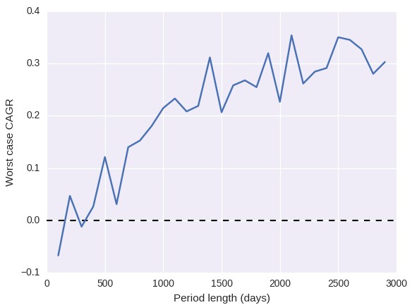
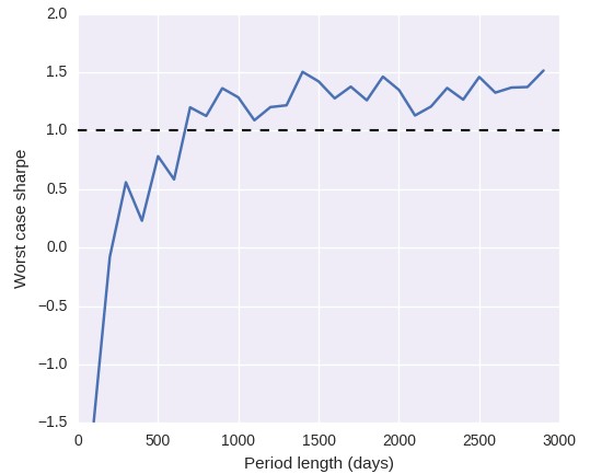
The code above shows how this works for a sample 30 year trading system results file (you can download the back-test here). In this case we simply load the system into a sample dataframe and we then use the qq-pat plot_mc_wc_evolution_sharpe and plot_mc_wc_evolution_cagr functions to calculate plots that show the evolution of the worst case sharpe and CAGR values for time periods from 100 to 3000 days in 100 day steps. You can use the max_period_length parameter to control how long you want to go and you can use the iterations parameter to control how many Monte Carlo simulations are done to draw results for each time period. In this case I used 50 simulations – which was enough to get convergent results – but you can use more if you want to get a graph that shows a cleaner trend in the evolution of the statistics. You can also use the code on some of my previous posts to load MT4 back-testing results data and perform the same analysis as well.

–

–

If you perform the above analysis you’ll notice that the first thing you get is the result of the get_mc_statistics function which gives you the Monte Carlo simualtion statistics for a time horizon equal to your back-testing period length (in this case around 28 years). For this system the worst case scenarios for a 28 year period are a cagr of around 40.8% and a sharpe of around 1.63. This means that if when you trade the system for 28 years and you have statistics below these values you can discard this system as having failed. However can’t we discard the strategy before that using a much better adjusted Monte Carlo scenario that matches the trading scenario we’re tracking live?

Using the qq-pat plot_mc_wc_evolution_sharpe and plot_mc_wc_evolution_cagr functions we can get the two plots showed above which show the evolution of the worst cases. As we would expect the initial worst cases are much lower – because short term behavior is much more random – but as the system continues to trade we see that our worst case expectation starts to turn positive. After around 500 days of trading both the Sharpe and CAGR are close to profitable territory – note that I used only 50 iterations so there is substantial noise in the measurement – but only at 1000 days are both the CAGR clearly above 0.0 and the Sharpe clearly above 1.0. From this point on the evolution of the system continues in a slower fashion, almost converging to the 28 year worst case values after 3000 trading days. Note that when I say “trading days” I mean days when the system has taken a position and obtained a given return.

–

–

The above functions provide a great tool for the evaluation of trading strategies and the real-time tracking of worst case scenarios using Monte Carlo simulations. Every time week you can perform a Monte Carlo simulation using the same period length as your current live trading results and you can very efficiently see whether you are above or below the worst case threshold. This makes it very easy to automate system discarding or to show you a red flag that can help you manually remove the strategy in question. Bear in mind that the analyzer.get_mc_statistics function also contemplates the period_length parameter. For example I can obtain the 99% confidence interval worst case statistics using 200 iterations for 300 trading days by using the call analyzer.get_mc_statistics(index=0, iterations=200, confidence=99, period_length=300).

If you would like to learn more about the determination of worst cases or you would like to become more experienced in the design, building and testing of automated trading strategies please consider joining Asirikuy.com, a website filled with educational videos, trading systems, development and a sound, honest and transparent approach towards automated trading.