During the past two posts (here and here) we have been discussing the use of Chaos theory to make predictions in financial time series. So far we have looked at different types of time series using a single fractal dimension calculation technique (“Rodogram”) and we have obtained some interesting results. Nonetheless there are some serious problems with the algorithm we have studied up until now, mainly problems dealing with the reproducibility of the results. On today’s post I am going to discuss these issues in more depth and I will be sharing with you a new implementation that eliminates these problems completely. As within the last two posts please remember that you need to have the quantmod and fractaldim R packages installed in order to reproduce these results. The code below shows the latest R implementation for the algorithm which does not contain the problems we will be discussing (to reproduce these issues you should use the algorithms published on the previous two posts).
–
library(quantmod)
library(fractaldim)

# Programmed by Dr. Daniel Fernandez 2014-2016
# https://Asirikuy.com
# http://mechanicalforex.com

getSymbols("USO",src="yahoo", from="1990-01-01")

# Predict the last 100 bars
endingIndex <-length(mainData$data)-101
mainData <- USO$USO.Adjusted
colnames(mainData) <- c("data")
TEST <- mainData[1:endingIndex]
total_error <- 0
error_per_prediction <- c()

#These are the fractal dimension calculation parameters
#see the fractaldim library reference for more info

method <- "rodogram"

Sm <- as.data.frame(TEST, row.names = NULL)

delta <- c()

# calculate delta between consecutive Sm values to use as guesses
for(j in 2:length(Sm$data)){
  delta <- rbind(delta, (Sm$data[j]-Sm$data[j-1])/Sm$data[j-1])
}

Sm_guesses <- delta

#do 100 predictions of next values in Sm
for(i in 1:100){

  #update fractal dimension used as reference
  V_Reference <- fd.estimate(Sm$data, method=method)$fd

  minDifference = 1000000

  # check the fractal dimension of Sm plus each different guess and
  # choose the value with the least difference with the reference
  for(j in 1:length(Sm_guesses)){

      new_Sm <- rbind(Sm, Sm_guesses[j]*Sm$data[length(Sm$data)]+Sm$data[length(Sm$data)])
      new_V_Reference <- fd.estimate(new_Sm$data, method=method)$fd

      if (abs(new_V_Reference - V_Reference) < minDifference ){
        Sm_prediction <- Sm$data[length(Sm$data)]+Sm_guesses[j]*Sm$data[length(Sm$data)]
        minDifference = abs(new_V_Reference - V_Reference)
      }
  }

  print(i)
  #add prediction to Sm
  Sm <- rbind(Sm, Sm_prediction)
  Sm_real <- as.numeric(mainData$data[endingIndex+i])
  error_per_prediction <- rbind(error_per_prediction, (Sm_prediction-Sm_real )/Sm_real )
  total_error <- total_error + ((Sm_prediction-Sm_real )/Sm_real )^2
}

total_error <- sqrt(total_error)
print(total_error)
plot(error_per_prediction*100, xlab="Prediction Index", ylab="Error (%)")
plot(Sm$data[endingIndex:(endingIndex+100)], type="l", xlab="Value Index", ylab="Adjusted Close")
lines(as.data.frame(mainData$data[endingIndex:(endingIndex+100)], row.names = NULL), col="blue")
–
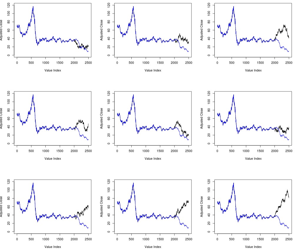
The problems within the past algorithm were highlighted by a comment made by Westh. In essence the issue is that the prediction results change whenever you run the code, showing that there is a substantial problem with the entire idea. There is definitely no point in making a prediction if whenever you make a prediction the prediction changes. The results you obtained could be extremely varied and therefore could simply fit the data if you run the simulation enough times. The image below shows you 9 different runs attempting to predict the last 500 days for the USO ETF. As you can clearly see there are all sorts of predictions from some that appear to be really spot-on to other predictions that are widely wrong. If running an algorithm multiple times can produce this sort of results then the results are meaningless.
Initially you would think that the problem is due to the lack of enough random samples in the construction of the guess – a poor construction of the distribution of potential values – but as Westh pointed out you obtain similar variability even if you increase the number of random samples to 5000, I tried increasing the random sample size to 20,000 and obtained very similar variability. The problem is due to the chaotic nature of the function that makes the predictions. The drawing from a normal distribution can produce a huge array of possible values and drawing even slightly different values for one prediction can lead to a different choice which then causes a change in the distribution which then reinforces the change and pushes the entire algorithm in a completely different direction. No matter how much you sample you will always find yourself within this predicament.
–
–
To make matters even worse the above phenomena ensures that the average actually never converges to anything but oscillates endlessly as a function of the number of simulations ran. So not only will two predictions always look different from one another but running many predictions does not give you anything more solid. The algorithm as presented within the last two posts was therefore useless in terms of actual market predictions since the values presented could change endlessly if the simulations were rerun. However once we understand the basis of the problem we can make some changes to be able to come up with a Chaos prediction algorithm – as the one included within this post – where predictions made are always exactly the same.
To eliminate the problem you must simply eliminate the source of randomness from the initial proposal made by Golestani and Gras within the original paper. This source of randomness was probably included to simplify the calculations but there is no actual need for it within the paper’s main idea. If the idea is that variations for a financial instrument should come out of the distribution of historical variations then the easiest fix for this problem is simply to use the actual historical distribution of returns as the source of guesses. So instead of drawing potential guesses from a normal distribution with potentially infinite variability we simply draw guesses from an array constructed from the finite return series derived from the original financial time series.
–
–
In this manner you can obtain the exact same result for the N consecutive runs of the same algorithm since the evaluation of the next best change is always going to be the same as there is always a single ideal candidate within the finite historical return series. In this manner we ensure that we always have a single choice that best minimizes the variation of the fractal dimension which ensures that our results are not going to vary on reruns of the same simulation. Of course the cost is much greater than previously because we explicitly evaluate all historical return candidates to see which one minimizes the variation in the fractal dimension but this is necessary to attain an algorithm that is actually useful for making predictions (at least to obtain an algorithm we can evaluate).
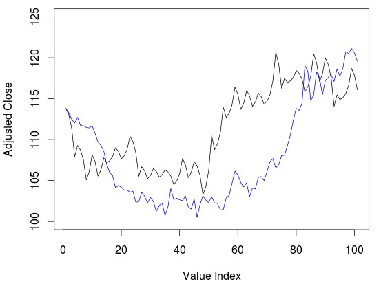
Sliedrecht The image above shows you the prediction for the past 100 days on the GLD ETF. This prediction is repeated in exactly the same manner whenever the algorithm is rerun. When running this new algorithm using the rodogram fractal calculation method results after 200 days do start to look significantly strange, reason why I decided to reduce the number of predictions to 100 on the latest algorithm. This may have to do with the exact fractal calculation method as my experiments using a few other methods have actually yielded better results (but this is something for a later post). That said as you can see the 100 day prediction on the GLD does look quite good although we have the presence of some strange dampening wave effect on the data – also commented by Westh – which I have confirmed is mainly due to the fractal dimension algorithm being used.
As you can see we now have access to a Chaos based prediction algorithm that is far more robust and which we can hopefully use to study things as actual prediction accuracy and different fractal calculation algorithms. If you would like to learn more about automated trading and how you too can build your own algorithms to tackle the markets please consider joining Asirikuy.com, a website filled with educational videos, trading systems, development and a sound, honest and transparent approach towards automated trading.