Mechanical Forex

Trying to predict which systems will come out as profitable under unknown future market conditions is the holy grail of algorithmic trading. If you could generate systems across some span of data and then say with a good confidence which ones would be profitable you would be able to constantly reap profits from the markets without having to worry too much about whether your systems would survive or not. However doing this is extremely hard – as I discussed within a past post – so it is expected that coming up with such a model would be extremely hard if not outright impossible due to changes in market conditions. Today we are going to look at how this model creation can be carried out, we will talk about the results of the created models and we will also talk about what would be required to arrive at a model that may work. You can download the data used in today’s post here.

–

library(randomForest)
library(caret)
library(e1071)
library(corrgram)
library(ggplot2)
library(rpart)

data <- read.csv("pathTodata/data.csv")
data <- cbind(data[,4:30], data[,57:58],  data[,31])
colnames(data)[30] <- "OSPtrade"
data$Custom.Criteria <- NULL

trainIndex <- createDataPartition(data$OSPtrade, p = 0.80, list = FALSE, times = 1)

efTrain <- data[trainIndex, ]
efTest <- data[-trainIndex, ]

r1 <- randomForest(formula = OSPtrade ~ ., data = efTrain,  ntree=100) 
plot(r1)

p <-ggplot()
p <- p + geom_point(size=3, aes(x=efTrain$OSPtrade ,y=predict(r1, efTrain), colour="Training set"))
p <- p + geom_point(size=5, aes(x=efTest$OSPtrade  ,y=predict(r1, efTest), colour="Testing set"))
p <- p + ylab("Predicted p-OS Profit (USD)") 
p <- p + xlab("Real p-OS Profit (USD)")
p <- p + theme(axis.title.y = element_text(size = rel(1.5)))
p <- p + theme(axis.title.x = element_text(size = rel(1.5)))
p <- p + theme(axis.text.x = element_text(angle = 45, hjust = 1))
p <- p + theme(panel.background = element_rect(colour = "black"))
p <- p + geom_abline(intercept = 0, slope = 0)
p <- p + opts(legend.position = c(0.9, 0.1))
p

–

The first thing you need to do to generate such a model is to have tons of different trading results. You should use a trading system generator to achieve something like this, for example like the open source openKantu software. For today’s experiment I have generated 500+ systems using EUR/USD daily data from 1986 to 2016. The systems were generated across 10 years of data and then pseudo out of sample tested for the following year. Note that the 10 year generation period for each system was chosen randomly and the 1 year pseudo out of sample period was the period immediately following each system’s in-sample data. This randomization of the in-sample period is fundamental as otherwise you could be looking at predictability that is localized across some set of market conditions, which might not hold significantly. Say if you always generate systems using data from 2000-2014 and then test for 2015, you could obtain a model that successfully predicts but only for those very specific conditions. All systems selected have an R² > 0.9 and a trading frequency above 10 trades/year across their in-sample period.

Once you get a set of systems generated under randomized in-sample periods the next step is to look at whether there are any relationships between the in-sample statistics and the pseudo out-of-sample results. Since we have many different statistics we can use random forests models to attempt to do this prediction as random forests are robust to high dimensionality and are not considerably hurt by having either duplicate or irrelevant variables. Granted any other machine learning model could be used for this purpose – with precautions specific to each case – but for today’s exercise we are going to be trying random forests. To create the random forests we use the randomForest R library and we then use ggplot to create our resulting graphs.

–

–

Another important thing to take into account is data splitting and model generation variability. When building this type of models you should always make sure you split your data into a training and a testing set to ensure that you have predicting ability outside of the data used to train the model. Traditionally you use most of the data – say 80% – for model building and then keep 20% for validation. Since this splitting is done randomly – attempting to preserve the distribution of the variable we want to predict between both sets – it is also important to do many split train/test sets and generate the model many times to ensure that your results were not spurious simply due to the way in which you split data sets and the random model generation but that you are indeed tackling a fundamental relationship between the variables.

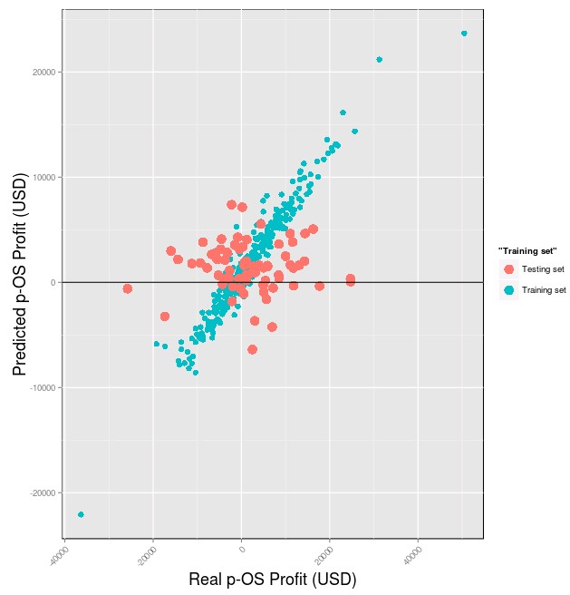
Some average results obtain with the above data and randomForest models are showed above. As you can see the model behaves very well within the training set – where it achieves an amazing ability to predict p-OS results – but under the testing set the model simply falls appart as it is unable to predict the p-OS result correctly. Success in model predictions are often best seen in the extremes of the data set as failures to predict more extreme values suggest that the model is simply unable to grasp any real relationship between the variables. In this case the most extreme values in the testing set – which have real p-OS values of around 20K and -20K – totally fail to be predicted with the predicted values being close to 0. A hallmark of failing models is that they always end up predicting the average, with deviations increasing as the values become more extreme.

–

–

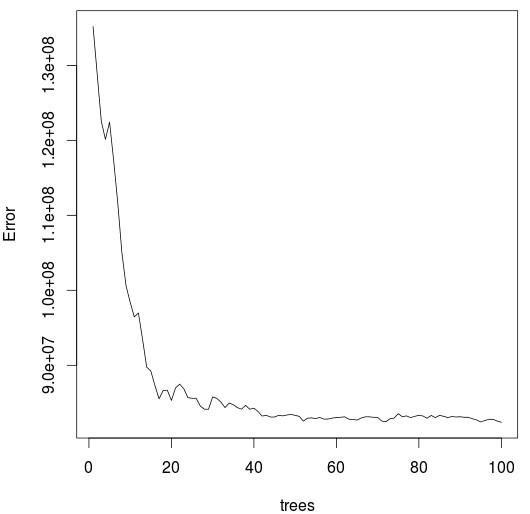
A look into the random forest training also reveals that training was carried out successfully, even though the number of trees used within the model is not significantly high. What happens here is basically what happens most of the time when trying to predict p-OS performance across any meaningful sample of systems, the in-sample variables are largely uncorrelated with the out-of-sample variables and any statistical variables related with the in-sample period appear to hold no predictive power. Of course the above is just an example of how this can be done using a sample data set and model type but the idea is that you design your own experiments and run your own attempts to attempt to see if you can indeed get to the holy grail and build a model that can adequately forecast p-OS performance. If you would like to learn more about algorithmic trading strategies and how you too can automatically create and trade systems please consider joining Asirikuy.com, a website filled with educational videos, trading systems, development and a sound, honest and transparent approach towards automated trading.strategies