Last week I talked about a random forest model that seemed to have a significant statistical edge in predicting the 6 month profitability of price action based trading strategies. This model was built using the R randomForest library and gave results that were able to significantly improve the average returns of randomly split cross-validation sets, meaning that the model was able to get a significant insight into relationships between in-sample and out-of-sample statistics. Today I want to talk about how this model compares to a similar model built using the python sklearn implementation of the random forest algorithm, which one performs better and which one I will be using going forward.
–

–
For this exercise I generated a database set containing 3591 strategies with 25 variables related with in-sample performance (back-testing statistics) obtained using data from 1986 to the time when each strategy was mined plus variables related with strategy characteristics (trading hour, stop loss, etc) and a classifier variable that measures whether the strategy was profitable or not six months after its creation. The strategies were mined from 2014 to February 2016 and therefore contain many different six month periods for out-of-sample performance. This is important as if all strategies shared the same out-of-sample period the probability for the model to only work for a given fixed set of market conditions would be greater. This data was randomly split into an 80% training set and a 20% testing set. Improvements in returns were measured by comparing the average return of trading the entire testing set and only trading those strategies that the model predicted would be profitable.
When generating the R/python models I used the same number of tress (200) and made no effort to optimize this number in any of the two implementations, all other characteristics were left at their default values. Since random forests have a random initialization I trained 100 models and obtained the average statistics to ensure that results were not due to simple luck from the model creation process. In general accuracy in predictions was similar between both models – around 57% – with the average return improving by roughly the same magnitude in both cases. In both cases the average return in the testing set improved by around 2-4 times compared with the return that would have been obtained without following any prediction. This is particularly because the models were good at removing big losing strategies.
–

–
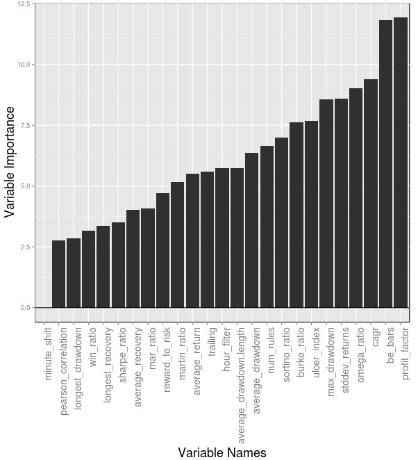
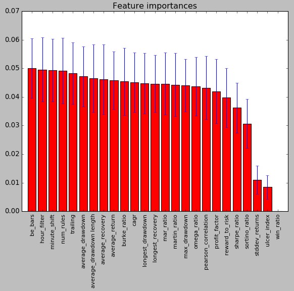
The two images above show the variable importance ranking for the models created in R (first image in the post) and Python (second image). As you can see it is rather surprising to see that the relevant variables are very different. In the case of the Python model the be_bars, hour_filter, num_rules and trailing variables are the most important while in the R case the most important variables are the profit_factor, be_bars, cagr and omega_ratio variables. The be_bars is the only variable in common in the top 5 between both models and some variables like the omega_ratio have a much lower importance in the case of the Python built model. It is surprising to note that the Python model ranks variables related with the actual strategies – rather than their past performance – highest. This is particularly valuable as it means that mining can probably be tuned to generate strategies that have a higher tendency to do well under real out-of-sample conditions. I would also like to add that the above importance rankings are almost the same for different model generation runs in R/Python.
Adding to the above I also tested the strategies on an incomplete OS set created using 1724 strategies that have less than 6 months of out of sample trading. The idea was to see whether the above models could improve results in this set, even though none of the strategies have yet to achieve the 6 month out-of-sample trading time that the models are expected to predict. The R model failed quite dramatically in doing this, making results worse by around 50%. This group of strategies had an average return of -0.0534% which became much worse (-0.0707%) when using the R model for predictions. The python model however proved to be more successful, improving the return slightly to -0.0513%. However given that the improvement was so small it may as well be attributed to random chance. It is worth noting that many of these strategies have just traded for a few months or even weeks, so there is a much larger randomness component than when trying to predict 6 month returns (the edges have had a much smaller time to show up). To properly evaluate the generated models we will need to have a set of mined strategies that reach 6 months of trading under conditions that were never seen by models within the original data set.
–

–
With the above I would say that the Python models seem to be better at what I want to do, although cross-validation performance was similar for both. Not only were the predictions in the incomplete set much better for the Python model but the variable ranking suggests that this model might be able to help in guiding strategy mining towards what might be more favorable targets. Another big advantage for the python model is that we can easily streamline it within our strategy mining filtering process given that this is already all done within the Python language. If you would like to learn more about system mining and how you too can trade large portfolios using thousands of trading strategies please consider joining Asirikuy.com, a website filled with educational videos, trading systems, development and a sound, honest and transparent approach towards automated trading strategies.


