There are many statistic currently available to traders that help compare strategies in terms of risk adjusted returns. Perhaps the most popular statistic during the past 40+ years has been the Sharpe ratio as its calculation is both easy to do and useful in terms of measuring the risk adjusted return of strategies. However many people have criticized the way in which the Sharpe ratio is calculated and have actually devised new statistics – such as the Sortino ratio – that attempt to circumvent its alleged problems. On today’s post I am going to talk about the Sharpe ratio, how it’s calculated, what the problems that are generally mentioned are and what implications these problems have when comparing strategies. We will also see why the use of the Sharpe ratio as a sole statistic is not ideal and which statistics can actually compliment the Sharpe ratio. I will also talk about some of the suggested improvements for the Sharpe ratio and which one I consider best.
–
–
$Sharpe Ratio = \frac{\rho_0-\rho_r}{\delta_0}$ (Equation 1)
–
The Sharpe ratio is often defined in the form showed by equation 1. In this equation rho sub zero is the average annual return of the system we’re interested in, rho sub r is the average annual return of a given reference risk-free return and delta sub zero is the standard deviation of annual returns for our system. In practice this equation is rarely used exactly as it is because the definition of a risk free return is arbitrary and therefore anyone could simply change this to make their Sharpe ratio bigger or smaller. For this reason almost everyone in the financial industry assumes that the risk free return is 0 and calculates the Sharpe ratio simply by dividing the annual average return over the standard deviation of annual returns. Note that the Sharpe ratio is usually defined using yearly returns, using any other period would necessarily imply a correction of the Sharpe ratio using a multiplication by the square root of the number of valid periods in a year. For example if you have daily returns you would multiply by sqrt(252) – trading days in a year – or if you had weekly returns you would multiply by sqrt(52) which are the number of weeks in a year.
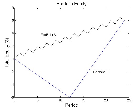
So what are the problems with the Sharpe ratio? Well the first problem we have is that the standard deviation and average return measurements do not care about the way in which returns present themselves. There is no accounting for how returns are distributed as a function of time, provided that in the end these two statistics give the same values. You can have two curves as in the above image (borrowed the chart from here) where you have two curves that have identical mean returns and standard deviations – therefore identical Sharpe ratios – but it is obvious that the Portfolio B curve is inferior to the Portfolio A curve. The most important weakness of the Sharpe ratio is therefore this lack of accounting for the level of correlation between time and returns.
–
–
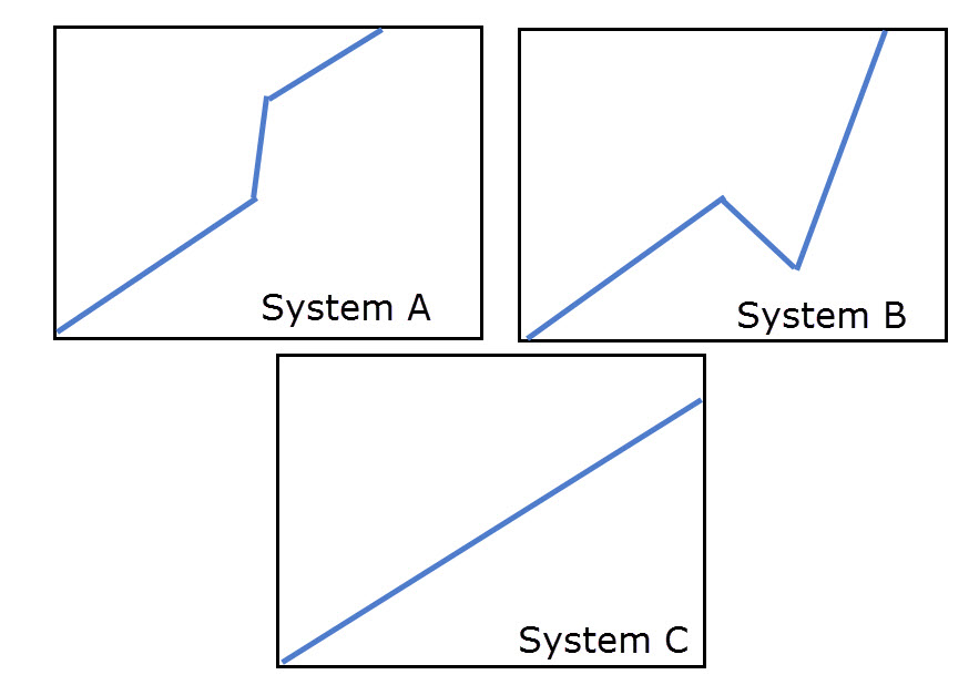
The second problem people often mention is that the Sharpe ratio does not care about the direction of deviation when measuring the standard deviation statistic. The Sharpe will judge systems A and B in the above image as being equally bad, although most people would recognize system A as being much better than system B. System A has a huge profit deviation while system B has a huge drawdown deviation so there is apparently no rational argument to trade B instead of A or to consider them on equal grounds. However in my view a system with an upside deviation that matches a system with an equal downside deviation – both having the same average returns – is equally bad because it implies a similar level of instability in the returns. If we had an equal system C with neither of these two deviations and the same average return it would indeed give us a much higher Sharpe which would put it as the definite champion between the three systems. These implies that the system that is less volatile is better than the system that is more volatile, even if such volatility happens towards the upside. I agree with this view as the Sharpe ratio rewards stability which implies less variability – in all manners – under all market conditions. We could all agree that it’s better to trade something with consistent returns than something that has more unpredictable returns.
Another important issue is the difference between the numerator and the denominator. The variation with the average mean return is linear while the variation with the deviation is hyperbolic. The use of the Sharpe ratio – and any other ratio for that matter – implies a disproportionate relationship between the numerator and denominator when comparing two trading strategies. The Sharpe ratio will always give much better scores for something with very low volatility compared with something that has higher returns. As the Sharpe ratio tends to infinity as the denominator becomes lower and lower, it is difficult to compare curves with equal returns and very low deviations. Since the accumulation of returns is also not linear but exponential you can also have cases where the mean return is positive but the net result of a strategy is negative. For a much more thorough analysis of these problems I suggest reading this page on Sharpe ratio problems and potential solutions.
–
–
Attempts to fix the above mentioned problems have resulted in the invention of new trading statistics. The sortino ratio is an attempt at changing the calculation to focus only on downside deviations, which means that in the above example A would be equal to C and better than B, but fails to address all the other issues mentioned above. A better statistic that was created in the last mentioned link is a modified Sharpe ratio that uses the normalized logarithmic returns instead of the average return (therefore eliminating the problems related with compounding) and it also uses the standard deviation of the difference between the price curve and a reference “ideal curve” as a way to account for all the other problems within the Sharpe ratio calculation. Since the “ideal curve” has a fixed defined value at each point in time it therefore eliminates the lack of time dependence in the original Sharpe ratio measurement. In this statistic the two portfolios on the first image would give different results, with Portfolio A having a much higher modified Sharpe ratio statistic.
If you still want to use the Sharpe ratio then all the above problems should point to the fact that you cannot use it on its own. You need to have other statistics that talk to you about time dependence in order to be able to properly gauge results. Filtering results first by the R² of the log(balance) Vs time curve allows you to evaluate only strategies that behave like Portfolio A, eliminating everything that does not have a strong correlation between balance growth and time.However you might consider changing your Sharpe ratio calculation to that mentioned above, even if it’s more complicated it will give you a much better benchmark with which you can compare the risk adjusted return of different trading strategies or portfolios.
If you would like to learn more about the evaluation of trading strategies and how you too can learn to compare and choose between different systems (or even create systems with a desired historical statistical value) please consider joining Asirikuy.com, a website filled with educational videos, trading systems, development and a sound, honest and transparent approach towards automated trading


