I have written in the past about the use of old market data (1985-2000) in the back-testing and design of Forex systems (for example here and here). There is a significant number of traders who believe that you should not use old data because it is “out-dated” and does not represent the “current market” and that changes in overall market structure during this entire time have caused extremely large changes in the market that make any conclusions drawn from experiments including this data completely irrelevant. Traders who hold this view commonly point to the raise of computer based trading and the rise of the internet as two reasons why both market structure and information flow are different and hence past market data should not hold any relevance in today’s market. The real question is, is this actually true? On today’s post we are going to take an evidence based approach to the testing of this hypothesis. We will look at the search for trading systems in old data (1986-2000) and we will see how much predictive value they actually hold across new market data (2000-2015). You can download the data that we will be using through the article here.
–

–
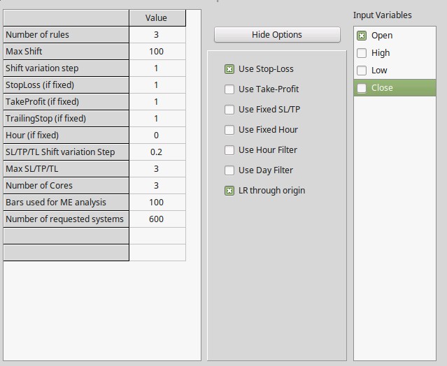
To see if old market data does hold any predictive value across the newer market data we must use statistical hypothesis testing. We establish the null hypothesis that past performance in the 1986-2000 set is not indicative of performance in the 2000-2015 set and we set to negate this null hypothesis. To do this we first establish the probability that a trading system with a high linearity (R²>0.95) and low max drawdown length (<500 days) generated across 15 years of random market data is profitable through the next 15 years and we see if the percentage of profitable systems on the average random data set (used more than 100 random data sets generated using bootstrapping with replacement) over the percentage of systems found on the real data set is less than 1%, if this is the case we can then negate the null hypothesis that 1985-2000 past performance is not related with 2000-2015 performance with a 99% confidence. For the generation process in OpenKantu I used the options showed on the image above.
–
#Load required libraries
library(ggplot2)

#loading data and eliminating columns that are not necessary
#change the paths below to point to the adequate files
eurusd <- read.csv("/pathtofile/eurusd_results.csv")
usdjpy <- read.csv("/pathtofile/usdjpy_results.csv")
gbpusd <- read.csv("/pathtofile/gbpusd_results.csv")

#set symbols
symbols <- c("EURUSD", "USDJPY", "GBPUSD")

# number of systems that are profitable in 2000-2015
profitable <- c(100*length(eurusd[eurusd$OSP.trade > 0, ]$OSP.trade)/length(eurusd$OSP.trade),
100*length(usdjpy[usdjpy$OSP.trade > 0, ]$OSP.trade)/length(usdjpy$OSP.trade),
100*length(gbpusd[gbpusd$OSP.trade > 0, ]$OSP.trade)/length(gbpusd$OSP.trade))

#number of systems that are better in 2000-2015
better <- c(100*length(eurusd[eurusd$OSP.trade >= eurusd$Profit.trade, ]$OSP.trade)/length(data[eurusd$OSP.trade > 0, ]$OSP.trade),
            100*length(usdjpy[usdjpy$OSP.trade >= usdjpy$Profit.trade, ]$OSP.trade)/length(data[usdjpy$OSP.trade > 0, ]$OSP.trade),
            100*length(gbpusd[gbpusd$OSP.trade >= gbpusd$Profit.trade, ]$OSP.trade)/length(data[gbpusd$OSP.trade > 0, ]$OSP.trade))

#put together dataframe
all_symbols <- data.frame(symbols, profitable, better)

#show table with all results
print(all_symbols)

#Profit/trade and OSP/Trade scatter plot with regression line
ggplot() +
  geom_point(size=2, aes(x=eurusd$Profit.trade, y=eurusd$OSP.trade, colour="EURUSD")) +
  geom_point(size=2, aes(x=usdjpy$Profit.trade, y=usdjpy$OSP.trade, colour="USDJPY")) +
  geom_point(size=2, aes(x=gbpusd$Profit.trade, y=gbpusd$OSP.trade, colour="GBPUSD")) +
  geom_smooth(method = "lm", data=eurusd, aes(x=eurusd$Profit.trade, y=eurusd$OSP.trade, colour="EURUSD"), formula = y ~ x)+
  geom_smooth(method = "lm", data=eurusd, aes(x=usdjpy$Profit.trade, y=usdjpy$OSP.trade, colour="USDJPY"), formula = y ~ x)+
  geom_smooth(method = "lm", data=eurusd, aes(x=gbpusd$Profit.trade, y=gbpusd$OSP.trade, colour="GBPUSD"), formula = y ~ x)+
  ylab("Profit per trade (2000-2015)") +
  xlab("Profit per trade (1986-2000)") +
  theme(legend.position = c(0.9, 0.15)) +
  theme(legend.title=element_blank())+
  geom_hline(yintercept=0)

#distribution of profits in 2000-2015
ggplot() +
  geom_histogram(aes(x=eurusd$OSP.trade, binwidth = 50, colour="EURUSD"), fill=I("blue"), alpha=I(.2)) +
  geom_histogram(aes(x=usdjpy$OSP.trade, binwidth = 50, colour="USDJPY"), fill=I("red"), alpha=I(.2)) +
  geom_histogram(aes(x=gbpusd$OSP.trade, binwidth = 50, colour="GBPUSD"), fill=I("green"), alpha=I(.2)) +
  xlab("Profit per trade (2000-2015)") +
  ylab("Frequency") +
  theme(legend.title=element_blank())+
  theme(legend.position = c(0.9, 0.8)) +
  geom_vline(xintercept=0, size=2, linetype = "longdash")
–
This mining process carried out on 100 random data sets generated using bootstrapping with replacement from each real data set generated on average less than 1% systems that were profitable within the second 15 year period data. The value is extremely low because the probability to be profitable across such a long time span becomes very low for a random walk process, which is essentially what happens if a system has no edge. This means that if we find that 20% of systems are profitable in the 2000-2015 period we would already be able to say that this is well above what is expected simply from random chance and that the 1988-2000 data actually holds information that is relevant for the prediction of profitability in the 2000-2015 period. We could say that old market data was not irrelevant.
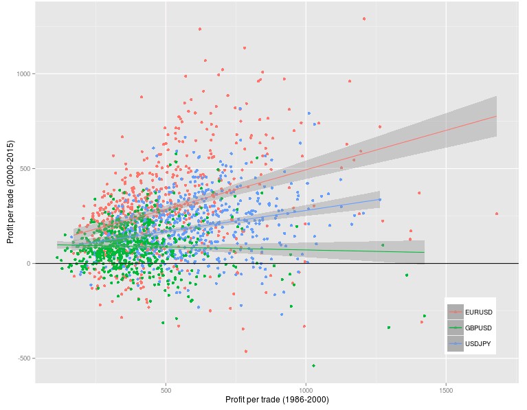
When we analyze the results from doing the above exercise on the EUR/USD (DEM/USD before 2000), USD/JPY and GBP/USD daily timeframes (3 pip constant spreads)(you can reproduce my analysis using the R script above and the data linked before) you can see that the probability to generate a strategy that was profitable in the 2000-2015 period is very high, as a matter of fact the probabilities are 88.5% (EUR/USD), 90.5% (USD/JPY) and 80.16% (GBP/USD) much higher than the expected probabilities from a simple luck of the draw. In fact the large majority of systems were able to make money in the 2000-2015 period which would be extremely improbable if the information present in the 1988-2000 period was simply irrelevant. There was an obvious deterioration in system quality under such a long out of sample period as systems only performed equally or better 20.7% (EUR/USD), 0.92% (USD/JPY) and 1.66% (GBP/USD) of the time but the mere fact that they were able to make money overall over this period is already fascinating.
–

–
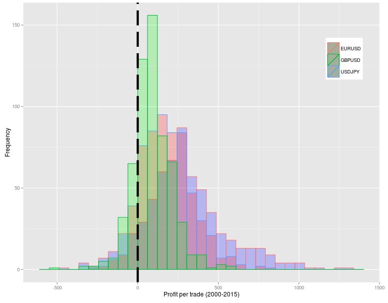
But what if losers were simply much worse than winners and it was all made up of small winners and huge losers in the 2000-2015 period? The analysis of the distribution of 2000-2015 results shows that this is actually not the case. The distributions show that losers are in general much smaller than winners on average with the distributions skewed heavily towards a larger profit/trade. This is completely unexpected if the 1988-2000 data was irrelevant because when no real inefficiencies are present in the data used for mining the future profit distributions are heavily skewed towards the losing side, as you would expect for a random walk process with a negative drift caused by trading costs. Repeating the above analysis for the EUR/USD 1H, 30M and 15M results yield extremely similar results so as a matter of fact this does not seem to be a timeframe dependent phenomena.
–

–
Despite what people like to say about old data not being useful and the market having changed, the reality is that old data, even data from 1986, holds important information that can lead to the creation of systems that survive newer and unknown market conditions. Why this is the case is certainly open to speculation but the truth is that old market data -despite the advent of the internet and computational power – transmits some general market characteristics that may still be useful today for the creation of profitable trading systems. If the 1988-2000 data was relevant to create profitable systems from 2000-2015 then it is reasonable to assume that it will also hold some relationship with the future 2015-2030 data. Using all available market information (1986-2015) for the creation of trading systems ensures that we reduce curve-fitting and only capture the most general of market inefficiencies.
In the end systems created using vast amounts of data (almost 30 years) may hold the greatest chances of achieving profitable results going forward as they contain the least amount of curve-fitting and the most information to tackle new market conditions. If you would like to learn more about system generation and how you too can create trading systems with low data-mining bias using GPU technology please consider joining Asirikuy.com, a website filled with educational videos, trading systems, development and a sound, honest and transparent approach towards automated trading.


