Mechanical Forex

On my first post about time series forecasting using chaos I showed you the R code I programmed to make some simple time series predictions using the methodology proposed within this 2014 nature paper. Today I want to continue with this post in order to further expand on the possibilities of Chaos based forecasting by using a similar to make some predictions on some other different symbols. On this post and a few subsequent posts we will be looking at the results of this method to make predictions on currencies, other stock indexes and commodities to see whether this methodology can yield accurate predictions on any of them. I will also talk a bit about measuring forecasting accuracy and how this method fares when we actually get some quantitative error measurements out of it. Please remember that to run the code showed within these posts you’ll need to have the quantmod and fractaldim R libraries installed. I also recommend the use of the RStudio software for an overall better R experience.

–

library(quantmod)
library(fractaldim)

# Programmed by Dr. Daniel Fernandez 2014-2016
# https://Asirikuy.com
# http://mechanicalforex.com

getSymbols("EWC",src="yahoo", from="1990-01-01")

# We want to predict the EWC after a given endingIndex
endingIndex <-3400
mainData <- EWC$EWC.Adjusted
colnames(mainData) <- c("data")
TEST <- mainData[1:endingIndex]
total_error <- 0
error_per_prediction <- c()

#These are the fractal dimension calculation parameters
#see the fractaldim library reference for more info

method <- "rodogram"

#number of samples to draw for each guess
random_sample_count <- 200

Sm <- as.data.frame(TEST, row.names = NULL)

#do 500 predictions of next values in Sm
for(i in 1:500){
  
  delta <- c()
  
  # calculate delta between consecutive Sm values to use for the 
  # building of the normal distribution to draw guesses
  for(j in 2:length(Sm$data)){
    delta <- rbind(delta, Sm$data[j]-Sm$data[j-1])
  }
  
  # calculate standard deviation of delta
  Std_delta <- apply(delta, 2, sd)
  
  #update fractal dimension used as reference
  V_Reference <- fd.estimate(Sm$data, method=method, trim=TRUE)$fd
 
  # create 50 guesses drawing from the normal distribution
  # use the last value of Sm as mean and the standard deviation
  # of delta as the deviation
  Sm_guesses <- rnorm(random_sample_count , mean=Sm$data[length(Sm$data)], sd=Std_delta )
  
  minDifference = 1000000
  
  # check the fractal dimension of Sm plus each different guess and
  # choose the value with the least difference with the reference
  for(j in 1:length(Sm_guesses)){
    new_Sm <- rbind(Sm, Sm_guesses[j])
    new_V_Reference <- fd.estimate(new_Sm$data, method=method, trim=TRUE)$fd
    
    if (abs(new_V_Reference - V_Reference) < minDifference ){      
      Sm_prediction <- Sm_guesses[j]
      minDifference = abs(new_V_Reference - V_Reference)
    }
  }
  
  print(i)
  #add prediction to Sm
  Sm <- rbind(Sm, Sm_prediction)
  Sm_real <- as.numeric(mainData$data[endingIndex+i])
  error_per_prediction <- rbind(error_per_prediction, (Sm_prediction-Sm_real )/Sm_real )
  total_error <- total_error + ((Sm_prediction-Sm_real )/Sm_real )^2
}

total_error <- sqrt(total_error)
print(total_error)
plot(error_per_prediction*100, xlab="Prediction Index", ylab="Error (%)")
plot(Sm$data, type="l", xlab="Value Index", ylab="Adjusted Close", main="EWC Rodogram")
lines(as.data.frame(mainData$data[1:(endingIndex+500)], row.names = NULL), col="blue")

–

On the first part of this series you saw the results of the Chaos prediction algorithm in the SPY within two crisis periods. I didn’t diagnose the error for these predictions and was just making some qualitative assessments over the possibilities using this prediction methodology. Today I want to further expand on this by looking at other symbols, mainly EWC, GLD and USO which cover different markets, for this I will use the code posted above. As you can see I keep using the “rodogram” methodology for the calculation of the fractal dimension but we will be testing other fractal dimension calculation methodologies on part 3 of this series of posts. Please note that predictions in all images are shown as black lines, blue lines represent the yahoo adjusted return.

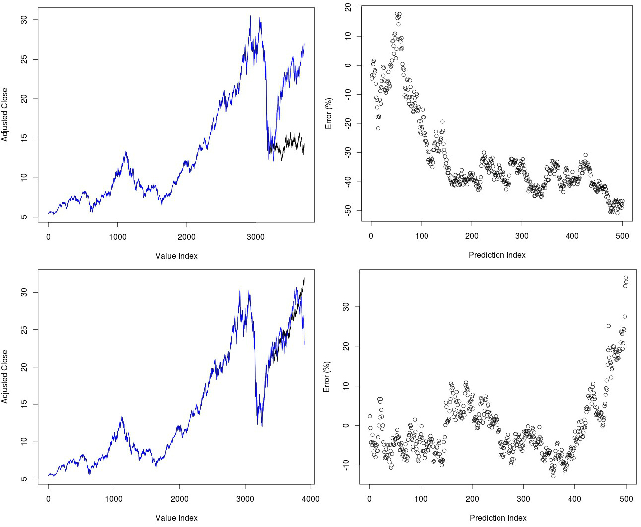
I want to start by looking at EWC predictions at different points in time. Since yesterday we predicted mainly crisis periods it is interesting to now look at whether the method can also predict rises after steep declines. We find within the top images below that predictions of the EWC within the 2009-2011 period right after the financial crisis are quite wrong. Although the chaos algorithm does not predict any further declines – actually predicting the low quite accurately in terms of magnitude – it does fail to predict the 50% rise that we saw within the next two years. If we see the error for predictions – calculated as the percentage difference between the predicted value and the real value in terms of the real value – we can see that errors increase significantly as time passes, reaching a -50% value near the end of the prediction period. Error are also not significantly small within the first 100 bars, swinging between +/-20% errors through this time. It is evident that errors can be large even at small lags.

–

–

If we shift the above prediction by 200 days we get a completely different picture (second set of images above). In this case the algorithm does predict a steep rise of the EWC but now fails to predict the decline that we saw in 2013. This failure to predict the decline shows as a steep rise in the accumulated error near the end of the test – after around 400 bars – leading to a 30% total error near the end. However it is quite remarkable that in cases such as this we get such an accurate prediction of directionality up to such a long time. Having a total accumulated error of +/- 5% after a two year run that increased the value of the instrument almost 50% is indeed a quite surprising feat. That said you can already see some of the important issues with the method, we might get very significant errors at small lags and our long term accuracy depends substantially on when we make a prediction. This hints that the best way to use this predictor might be to make a medium term prediction and only making a bet if there is significant directionality within it (if the algorithm predicts a sharp decline or rise).

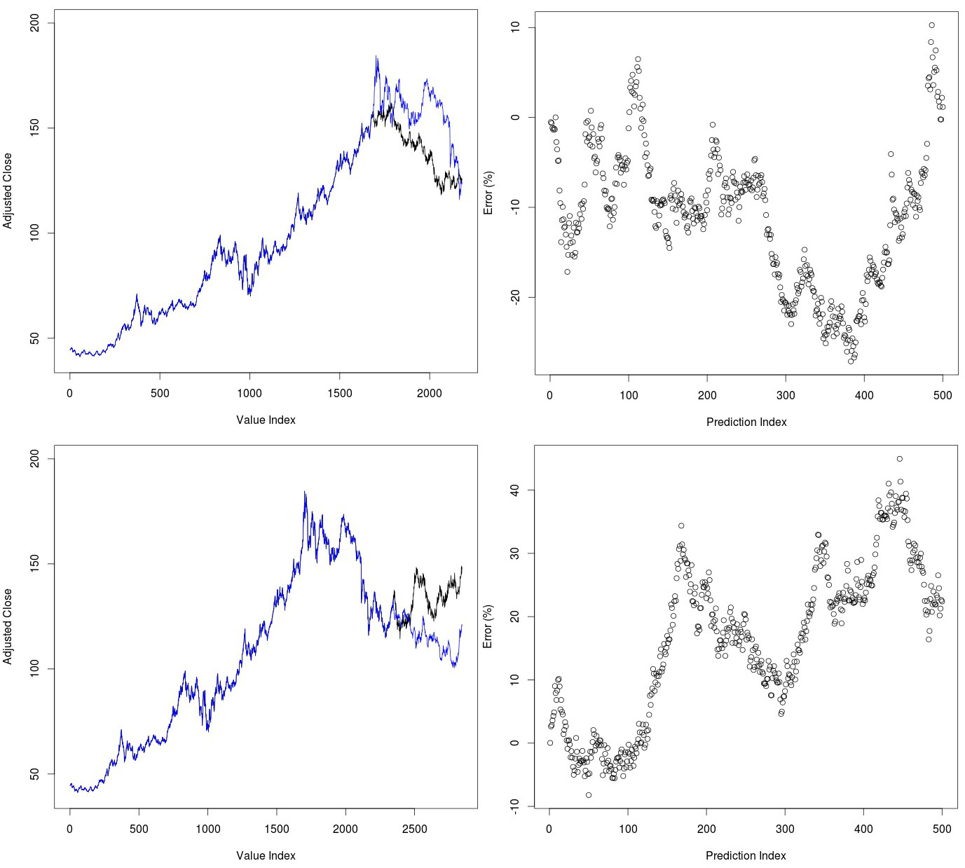
Gold is also a very interesting case because it moved within a steep uptrend during the 2000-2013 period and only suffered a significant decline within the 2013-2016 period. We can see whether our algorithm was good enough to predict the crash in GLD and whether it was able to predict the recent rise that took place during the recent past. The images below show both prediction cases for GLD. The predictions for gold after it reached its high in 2011 are quite amazing. Despite the fact that the algorithm had a time series where no declines of such magnitude had ever been present the algorithm predicted the decline in gold with good precision during the next few years. As you can see errors were most significant during the middle of the test but the evolution of the price series was such that both ended up matching close to the end of the prediction period. Predictions for the recent past were less successful. The algorithm failed to predict the decline in gold prices after around 100 days and started to accumulate very significant errors, reaching an even 40% mismatch with actual gold prices. This further supports the point that you have to see a very strong move within the Chaos prediction in order to have some expectation of success.

–

–

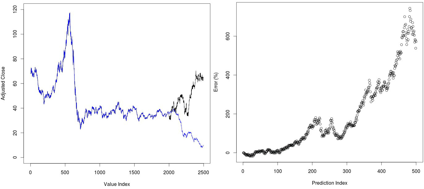
Another interesting case to look at is the recent decline of oil prices during the past year and a half. We can test whether our Chaos based algorithm is able to predict the USO price decline within the recent past. As you can see in the image below this prediction fails very dramatically, predicting practically the complete opposite to what happened in the ETF. This is the only case where I have witnessed such a dramatic failure of the Chaos based prediction mechanism and this may well be because USO does not follow the same rules as the other ETFs we have examined. For example it may be that the fractal dimension within the USO series is not preserved as a function of time and this leads to extremely bad predictions. This points out that measuring the actual historical variation in the fractal dimension within a series may be a good indicator of whether this method can yield reliable predictions.

–

–

Of course, as I have highlighted before, this is just the tip of the iceberg and does not really represent a rigorous quantitative evaluation of the merits of this algorithm. In order to do this it becomes necessary to perform systematic predictions at all possible different lags and evaluate the overall accuracy at each different point in time as a function of the entire history of the instrument being evaluated. This takes a lot of time but I am indeed currently carrying out such an experiment. If you would like to learn more about financial time series and how you too can create systems to trade in the markets please consider joining Asirikuy.com, a website filled with educational videos, trading systems, development and a sound, honest and transparent approach towards automated trading.