Earlier this year I wrote a post about the limitations in the reduction of portfolio drawdowns that are caused by the uncertainties inherent to short term returns. Today I want to go a bit deeper into this issue using quantitative simulations in R in order to figure out which approach might be more efficient to reduce portfolio drawdowns. The idea of these simulations is to provide some clear guidance into what type of systems need to be mined in order to achieve this goal and whether the limitations I mentioned before are really insurmountable or if something can actually be done to take portfolio drawdowns to even lower levels. You will be able to reproduce the simulations using the R code below.
–
#Coded by Daniel Fernandez 2016
#http://mechanicalforex.com
#https://asirikuy.com

all_mean_max_dd_length <- c()
total_simulations <- 100
max_systems <- 100
drift = 0.05
variance = 5.0

for(j in 1:(max_systems/5)){

total_systems <- 5*j
mean_max_dd_length <- 0

for(i in 1: total_simulations){
  portfolio <- c()
  for (x in 1 : total_systems) {
    rw <- cumsum(rnorm(n=7560, mean=drift, sd=sqrt(variance)))
    if (x == 1){
      portfolio <-  rw/total_systems
    } else {
    portfolio <- portfolio + rw/total_systems
    }
  }

  max_dd_length <- 0
  dd_length <- 0
  max_balance <- portfolio[1]

  for (x in 1: length(portfolio)){
    if (portfolio[x] > max_balance){
      max_balance <- portfolio[x]
      dd_length <- 0
    } else {
      dd_length <- dd_length + 1
      if (dd_length > max_dd_length){
        max_dd_length <- dd_length
     }
    }
  }

mean_max_dd_length <- mean_max_dd_length + max_dd_length/total_simulations
}
print(j*5)
all_mean_max_dd_length <- rbind(all_mean_max_dd_length, mean_max_dd_length)
}

system_values <- seq(5, max_systems, by=5)

exponential.model <- lm(log(all_mean_max_dd_length)~ log(system_values))
exponentialRegression <- exp(predict(exponential.model, list(log(system_values))))
plot(system_values, all_mean_max_dd_length, xlab="number of systems", ylab="Max drawdown period length", main=paste("variance", variance, "drift", drift))
lines(system_values, exponentialRegression, col="red")
–
In order to simulate portfolios we first need to think about how to generate trading strategies that are similar to those we use in real life. Trading strategies can be thought of as random walks with positive drifts that we can simulate easily using the R language. We can then play with two fundamental variables in the creation of these systems, the magnitude of their drift component and the magnitude of their variance. We can then create different numbers of these systems and put them together into equally weight portfolios and see how much the maximum drawdown length changes as a function of the number of systems. Looking at the variations within these results we can then figure out whether we should worry more about increasing the drift component of our strategies or reduce their variance. We can also see if neither of these have an effect or whether both are equally important.
Using the code above you can perform this type of simulations. The total_simulations variable determines the number of simulations done per system number (because we need to generate lots of portfolios from the same number of systems to reach convergent results) and the max_systems determines the maximum number of systems that will be contained within portfolios. The code performs portfolio simulations in 5 system steps, from 5 systems to the maximum number of systems you have specified. After that the program then plots the maximum drawdown length as a function of the system number as well as a power law regression (in red). Using this power law you can then predict the drawdown reduction at any given system number N if you wish to do so. You can also change the drift and variance as you wish. I have set the number of “days” in the simulation to 7560 which is representative of the 30 years we usually use in back-testing (252 business days times 30).
–

–
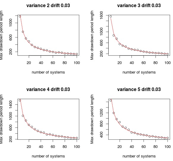
The simulations above already show that variance reductions have a rather limited effect in making the portfolio better. Taking the variance from 2 to 5 at a constant drift only reduces portfolio maximum drawdown lengths at 100 systems slightly, although it is quite clear that higher variances have a very significant effect on the drawdown values in small portfolios (below 50 systems). Variance reduction seems to play a rather limited role in the reduction of maximum drawdown lengths although it certainly reduces maximum drawdown lengths to some extent.
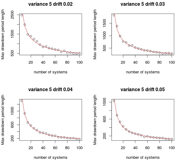
The drift component has a much more prevailing influence as you can see on the plot showing different drift values and a constant variance of 5. Decreasing the drift component by 30% immediately increases maximum drawdown lengths and the effect on drawdown lengths at low system numbers is even more dramatic than for the variance. The reduction in the maximum drawdown length is initially around 50 days for each 0.01 increase in the drift, to reach a maximum drawdown length below 50 days it is required to have a drift of 0.1 with a drift of 0.2 taking the maximum drawdown length at 100 systems to a value below 30 days. In this sense it becomes clear that the quickest route to reduce portfolio drawdowns would be to increase the drift – the mean return – of the strategies at hand. Reducing the standard deviation also helps but achieving the same below 30 day maximum drawdown requires a standard deviation of 0.1.
–

–
In the end the limits of potential in-sample maximum drawdown length reductions are set by the limits in the quality of the inefficiencies that can be found. Increasing the number of systems always allows you to get into lower maximum drawdown values but the standard deviation and return of the strategies limits how efficient this process can be. The fact that maximum drawdown reductions as a function of system numbers are dictated by power laws suggests that much larger numbers are needed to achieve the same drawdown reduction when lower quality systems are used. However this might be the only solution if there is a natural limitation to the number of very high Sharpe ratio inefficiencies that can be found in the market. Since in live trading we also face the issue of system failure it may also be a protection to use large numbers of systems instead of very few systems with very high historical Sharpes. This is even clearer if we consider that I have found no evidence that higher Sharpes in back-testing have a higher probability to lead to profitable live trading results (see this post). Although there is a minimum Sharpe for viable strategies, selecting higher Sharpe values than these does not seem to yield one year profitable results with a any higher chance (of course I am aware this may change as longer term results are accumulated).
This study shines some additional light into what actually causes portfolio maximum drawdown lengths to become smaller. It is a quality that can be enhanced by adding systems or by mining better systems but care must be taken since in real trading we must also consider the potential for system failure. Therefore we must use systems that are of a high enough quality – allowing to reduce maximum drawdown lengths as fast as possible – but also of enough quantity such that we have a lower selection bias when trading, which reduces the exposure to strategy failure. If you would like to learn more about system mining and how you too can create trading strategies automatically please consider joining Asirikuy.com, a website filled with educational videos, trading systems, development and a sound, honest and transparent approach towards automated trading.


