Today we continue our search for better large scale portfolio optimizations using traditional optimization techniques. After concluding that mean/variance optimizations usually lead to worse pseudo out of sample performance and also confirming that minimum variance optimizations have a reasonable expectation to out-perform naively optimized portfolios under market conditions where systems correlations change but system performance remains intact I now want to show you the results of another interesting test: changing the frequency of the returns used for the calculation of the optimization. I will first explain why this change makes sense and we will then go into the quantitative results I have obtained when using minimum variance optimizations using daily instead of monthly returns.
–

–
There is a big problem in traditional optimization techniques when the number of assets in the portfolio is bigger than the number of returns available. For example if you’re using monthly return data for 30 years you basically have 360 data points which means you can expect to get somewhat reasonable covariance matrix estimations up to around this number of assets. If you have much more assets than you have returns, say a 4000 system portfolio with the same return length, then you run into important covariance estimation errors due to the mathematical nature of the problem. As we have discussed in the past the solution to this problem has been to use techniques such as covariance shrinkage, or even more creative mechanisms such as the one showed within this paper. This last paper works exclusively in cases where the number of assets is much larger than the number of returns.
Another potential solution to the above issue is to simply fix the problem by going into a finer degree of detail within the assets being evaluated. For example you can go to daily returns instead of monthly returns which gives you a 30x increase in the number of returns you have available. If you go from monthly to daily returns you will no longer have 360 but nearly 91,000 returns. This means that covariance matrix estimation is most likely not going to be a problem up to the point where you have extremely large portfolios. However the main problem is that systems – unlike other assets like stocks – tend to have lots of zero return values in a daily resolution which means you can have strong covariance matrix estimation problems simply due to the amount of zeros within the returns matrix.
–

–
To reduce the above problem I decided to only use daily return data where at least one system had a non-zero return. Due to the high diversification present within our portfolio this included more than 70,000 days in all cases. The data was then divided into in-sample and pseudo out of sample data from 1986 to 2001 and from 2001 to 2016. The first data set was used to perform portfolio optimizations while the second set was used to measure the portfolio Sharpe using the weights obtained during the first period.
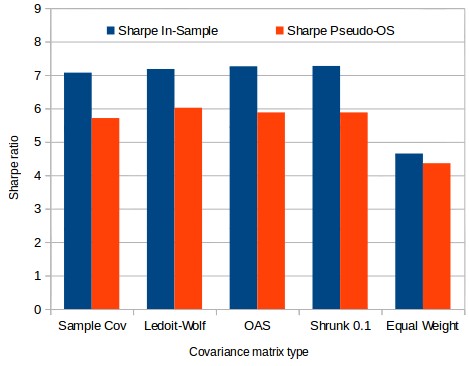
I was pleasantly surprised by the initial results obtained between in-sample and pseudo out of sample Sharpe ratio values. The first image above shows the in sample and pseudo out of sample Sharpe values for a 4000 system portfolio. As you can see the minimum variance optimization still overestimates the Sharpe significantly – due to estimation errors inherent to the changes in the covariance matrix as a function of time – but the overestimation is much smaller than in previous cases. In this case the over-estimation was in all cases around just 20% which is rather small compared to the values closer to 200% we were sometimes obtaining before. As we would have expected the equal weighted portfolio still provides the least difference between the in-sample and pseudo out of sample sharpes.
–

–
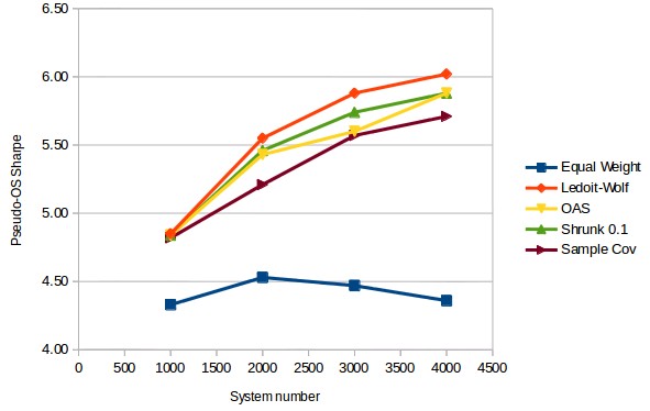
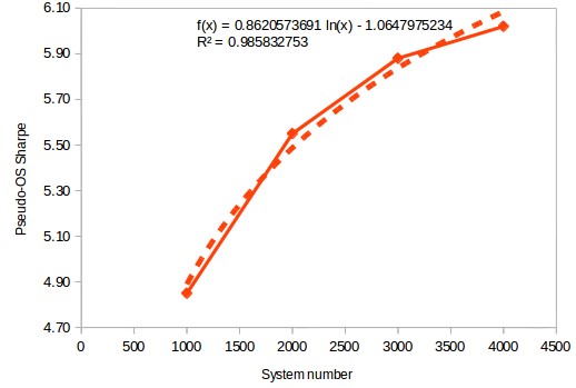
The most interesting results actually pertained to how the Pseudo-OS Sharpe between the minimum variance optimization and the equal weight optimization compared. Contrary to the monthly optimization case – where results were worse than the all-equal up until the 2000 system portfolio size – in this case we see that results are much better than the all-equal portfolio from the 1000 asset portfolio. As a matter of fact at this point the all-equal Sharpe remains rather constant as a function of the number of systems while the minimum variance optimization Sharpe increases – seemingly following a logarithmic curve – as a function of the portfolio size. The third image within this article shows the minimum variance optimization’s pseudo out of sample Sharpe using the Ledoit-Wolf covariance matrix estimation method along with a logarithmic regression. Following this curve we would expect to have a pseudo OS Sharpe near 7.47 at a system size of 20K and 8.76 at a system size of 90K.
The above results show that the variance minimization optimization using covariance shrinkage methods is expected to give the highest improvement against the equal weight optimization. At the current portfolio size (around 4400 systems) we would expect the long term out of sample Sharpe to be more than 50% greater than the long term sharpe for the equal weight portfolio. Of course whether this holds true or not will depend on how many of these systems fail and how long it takes them to do so — as all systems inevitably fail at some point. If you would like to learn more about portfolio optimizations and how you too can trade setups like these please consider joining Asirikuy.com, a website filled with educational videos, trading systems, development and a sound, honest and transparent approach towards automated trading.strategies


