One of the most important measurements when deciding what to trade is correlation. Building a trading system portfolio with strategies that are highly correlated is a recipe for failure since your strategies will all face drawdowns at similar times and your protection from strategy down-turns will be reduced compared to a properly diversified portfolio where strategies are sparingly correlated. On today’s post I want to show you how you can carry out this analysis in practice using Python. We will calculate global as well as rolling correlations for a group of four trading strategies. By using the code within this script you will then be able to diagnose the relationship between your trading strategy returns and build portfolios with strategies that only have low correlations. To reproduce the graphs within this post please make sure you download this sample system files.
–
#!/usr/bin/python
import sys
from datetime import datetime
import pandas as pd
import csv
import matplotlib.pyplot as plt

ROLLING_CORRELATION_WINDOW_SIZE = 12

def lastValue(x):
    try:
        reply = x[-1]
    except:
        reply = None
    return reply

def main():

    backtestFileList = ["sys1.txt", "sys2.txt", "sys3.txt", "sys4.txt"]

    j = 0

    for item in backtestFileList:

        print item

        tradeTimes = []
        tradeBalance = []

        with open(item, 'rb') as csvfile:
            reader = csv.reader(csvfile)
            i = 0
            lastBalance = 100000
            for row in reader:
                if i > 0:
                    if row[10] != "inf":
                        tradeTimes.append(datetime.strptime(row[3], '%d/%m/%Y %H:%M'))
                        tradeBalance.append(float(row[10]))
                i += 1

        loaded_series = pd.DataFrame(data=tradeBalance, index=tradeTimes).resample('M', how=lastValue).pct_change(fill_method='pad').fillna(0)

        loaded_series.columns = [item]

        if j == 0:
            allTimeSeries = loaded_series
        else:
            allTimeSeries = pd.concat([allTimeSeries, loaded_series], axis=1)

        j += 1

    allTimeSeries = allTimeSeries.fillna(0)
    correlations = allTimeSeries.corr()
    fig, ax = plt.subplots(figsize=(12,9), dpi=100)
    heatmap = ax.matshow(correlations, aspect = 'auto', origin = 'lower', cmap ="RdYlBu")
    ax.invert_yaxis()
    ax.xaxis.tick_top()

    plt.show()

    print allTimeSeries

    for index_1, system_returns_1 in enumerate(allTimeSeries.columns):
        for index_2, system_returns_2 in enumerate(allTimeSeries.columns):
            if (index_1 > index_2) and (index_2 != index_1):
                rolling_correlation = pd.rolling_corr(allTimeSeries[system_returns_1], allTimeSeries[system_returns_2], ROLLING_CORRELATION_WINDOW_SIZE)
                fig, ax = plt.subplots(figsize=(12,9), dpi=100)
                ax.plot(rolling_correlation.index, rolling_correlation)
                ax.set_title("Rolling correlation between systems {} and {}".format(index_1+1, index_2+1))
                ax.set_xlabel('Time')
                ax.set_ylabel('Rolling Correlation')
                plt.show()


##################################
###           MAIN           ####
##################################

if __name__ == "__main__": main()
–
The Pearson correlation measurement is a mathematical tool that helps us determine the degree of linear relationship between two variables. If two variables have a high correlation then a variation in one has been historically related with a variation in the other variable. In the case of trading systems a high correlation in strategy returns implies that the strategies are trading using similar market instruments or triggering behavior. Two trading systems that follow daily timeframe trends on the same instrument – even when using different indicators – are expected to be correlated to some degree since trends happen at the same time and therefore if both systems have been able to exploit them they must share some degree of correlation. We would want to avoid trading two strategies that have a high correlation in returns, since this implies that trading both is alike trading the same strategy with an increase in risk.
Correlations are however more complicated since there is more than one way to calculate them when talking about trading strategies (read here for more information). In general I calculate them using monthly returns, since this gives the most meaningful measurement as how different systems relate to different market conditions. Using shorter term correlations makes systems naturally appear more uncorrelated — as you can see in the linked post before. In the script shared above the correlation is calculated using monthly returns as well but you can change this by changing the resampling frequency in the pandas dataframe loading line (line 41) from “M” (monthly), to “D” (daily) or “W” (weekly).
– –
–
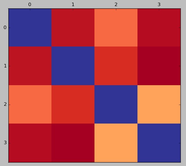
The script above first calculates a correlation map which is a useful tool that tells you the global correlation value between the strategies. You can hover your mouse over the values when the matplotlib dialogue opens to see the value for each different square. In the above example all systems share a low correlation with the highest correlation being between systems 3 and 4 at a value of 0.266. This means that these strategies are largely uncorrelated in their monthly returns meaning that they hedge each other’s performance quite well. When evaluating a group of trading strategies the global correlation maps are a good way to identify groups of more or less related strategies and also to discard strategies that may already be largely correlated to systems that have already been created in the past.
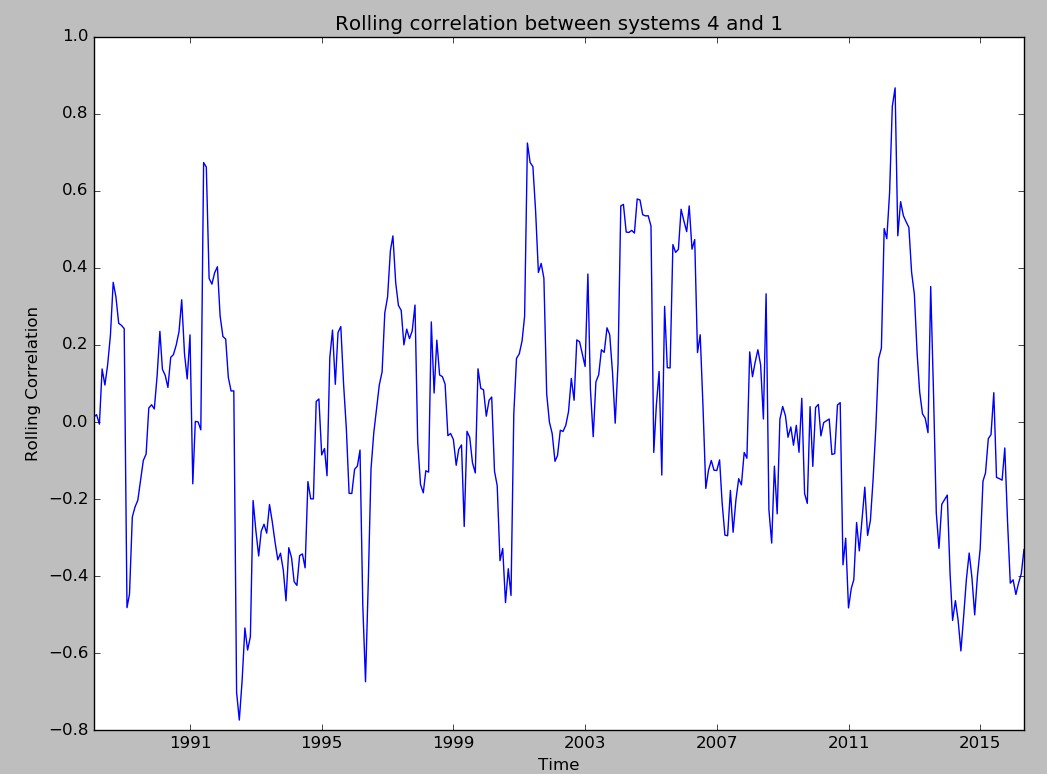
Additionally the script also calculates the system-by-system 12 month rolling correlation (you can adjust the window size by changing the literal constant in the beginning of the script). This provides a deeper piece of information since it allows you to see how the monthly correlation has varied between each system pair as a function of time. In the example below you can see that although system 4 has a very low global correlation with system 1 – as seen in the correlation map – the maximum value for the rolling correlation is actually quite high, at close to 0.8. This means that although the strategies remain largely uncorrelated most of the time there are specific periods where the strategy correlations might spike significantly. You might want to control the standard deviation of the system-by-system correlation or you might also want to limit the maximum spike that any system pair within your portfolio has seen.
–

–
Of course the above script works only for the system file format that we use at Asirikuy – used by the included sample files – but you may alter the script to load MT4 back-test or strategy result files in any other formats. It is just a matter of changing the balance and time loading code in the system loading loop. You might want to take a look at some of my previous posts related to MT4 system analysis to learn more about how you can easily parse htm files resulting from back-tests using this platform. If you would like to learn more about system analysis and how you too can trade large portfolios of uncorrelated strategies please consider joining Asirikuy.com, a website filled with educational videos, trading systems, development and a sound, honest and transparent approach towards automated trading.strategies


I had to modify one of the lines:
with open(item, ‘rt’) as csvfile:
to fix _csv.Error: iterator should return strings, not bytes (did you open the file in text mode?)