During my recent quest for machine learning based mechanisms to improve out-of-sample trading performance I have built a model that is able to classify systems when they are mined to select systems with higher chances of success for the first 6 months of out-of-sample trading. However this model has the limitation that it works only for systems right after they are mined and there is no way to update classification results after the model finishes the first 6 months of live trading. Today I will talk about a new model that compliments this implementation and is able to provide continuously updated predictions after the first three months of live trading. I will discuss some of the characteristics of this model, how it is different from the other model and how we hope it will increase our current live trading performance.
–

–
The first classification model I have developed used data from the in-sample performance of trading strategies in order to figure out whether systems that are added to our repository are worth trading for the first six months. This model was able to reach successful classification results under unseen data and is now implemented within our servers to give predictions on newly added strategies. The problem with this model is simply that it only works on newly added systems and it is of no value to strategies that have already accumulated an important amount of out-of-sample trading. This model is therefore of no value to making trading decisions after a system has already spent a significant amount of time in trading, making it necessary for us to develop a specialized model for this purpose.
With this in mind I developed a model that uses data from the out-of-sample trading of strategies to predict the results of their next three months of out-of-sample trading. To train this model I took strategies that had more than 3 months of out of sample trading – meaning they have live traded for at least 3 months – and extracted as many non-overlapping 3 month out-of-sample evaluation and 3 month out-of-sample target periods as possible. This means that a system that has been trading for 9 months could yield 2 points for the training data set (first point statistics for months 0-3, live results for 3-6, second point statistics from 3-6 and live results from 6-9). For the evaluation sets I calculated some basic statistics for prediction (sharpe, mar, omega, etc) and also included system related statistics (symbol, SL, TP, etc).
–

–
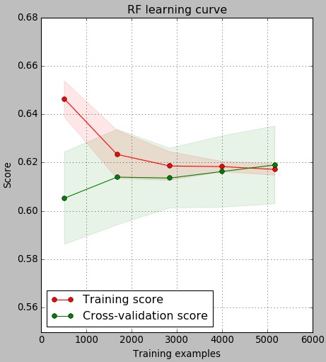
Given the above we currently have more than 5000 examples for training. The learning curve above shows how the accuracy of predictions – total number of values predicted to belong to the proper class – changed as the number of examples used in training increases. Remember that 10 models were trained for each point in this graph, preserving 20% of data for the testing curve evaluation in each case. As you can see substantial improvements in testing set performance happen till around 3000 examples while after that we have a slow but steady increase in accuracy for both testing and training sets. As with our previous classifier the learning curve shows the typical behavior of a complex problem where testing/training set accuracy tends to converge as the number of examples increases yet the values still suffer from a significant bias given the difficulty of the problem.
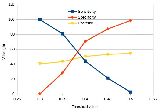
In analogy to our other model we can also choose the prediction boundary for the classification of a system as either profitable or unprofitable for the next three months of OS testing. You can see the values for sensitivity and specificity across testing sets when the threshold for classification is changed. At a prediction boundary of 0.3 we basically have all systems added – sensitivity is 100% – with the posterior probability being the regular probability to have a profitable 3 month period in the testing set (which is close to 40%). As the threshold increases the posterior probability increases as well – meaning that we gain insights into the data – with the highest posterior probability going above the 50% mark.
–

–
In terms of the relative improvement in returns on testing sets we can see that our results improve significantly as the specificity increases up to a value of around 0.45 where we have a sensitivity of around 20%. In contrast with the other model having higher specificity values is heavily detrimental with improvements in average returns dropping dramatically after the 90% specificity mark. It is worth noting that the relative increase in the OS profitability in this case is higher than 5x, meaning that the OS results when using the classifier are markedly better than those of the unclassified testing set. The insights we get are good enough to turn average negative result testing sets into positive average return testing sets after classification.
The idea is to use this model to classify systems every week to determine whether they will or will not be profitable during the following three months and trade only systems for which the classification is positive. This model therefore serves as a continuous classification algorithm for systems after their initial OS period and greatly compliments our initial addition classification model that looks just at in-sample trading data to decide whether or not to trade a system live during that initial period. In later posts we will discuss more about this model and how it affects the makeup of our current massively parallel portfolio. If you would like to learn more about our trading and how you too can trade portfolios containing potentially thousands of systems please consider joining Asirikuy.com, a website filled with educational videos, trading systems, development and a sound, honest and transparent approach towards automated trading.strategies.


