Mechanical Forex

On a previous post we learned how to perform a Markowitz portfolio weight analysis using the R statistical software and the PerformanceAnalytics, fPortfolio and quantmod packages. Using this analysis we learned how to obtain optimum historical system weights to reduce portfolio variance and increase overall performance. Today we are going to learn how to take this an additional step further in order to perform a portfolio weight analysis in which a portfolio is periodically rebalanced using Markowitz portfolio theory. While our first method seeks to answer the question of what the optimum historical portfolio weights would have been, our current analysis will seek to answer the question of what performance would have been like if a rebalancing scheme had been applied in the past with a certain frequency. Through the following posts I will show you how you can carry out this analysis in R and what information we can get from these results. By applying this analysis we’ll be able to see the weight evolution of our systems as well as an approximation to the historical portfolio performance. As always I recommend RStudio to perform this analysis.

–

systemList <- c()
systemList$systems <- c()
systemList$systemFileNames <- c()
systemList$systems <- c(systemListTest$systems, "system 1")
systemList$systemFileNames <- c(
systemListTest$systemFileNames, "C:/PathToFile/results.csv")
systemList$systems <- c(systemListTest$systems, "system 2")
systemList$systemFileNames <- c(
systemListTest$systemFileNames, "C:/PathToFile/results2.csv")
systemList$systems <- c(systemListTest$systems, "system 3")
systemList$systemFileNames <- c(
systemListTest$systemFileNames, "C:/PathToFile/results3.csv")

–

In order to carry out this analysis the first thing we’re going to do (showed above) is to create a list object containing our portfolio names and file paths, this is done in order to allow us to load N systems into the portfolio analysis since ideally we want this code to be as functional as possible. In the example above I have added 3 different systems (each file with one date and one balance column) and I have named them “system 1”, “system 2” and “system 3”. You can add as many systems as you want, just remember to add the system name to the systemList$systems list and the path to the systemList$systemFileNames list. Once you have done this we can now proceed to the portfolio calculations. First of all we load the libraries and create a portfolioXTS object containing all of our system results (showed below). After running this code you will have a chart showing the performance of all your systems plus a portfolioXTS object that we’ll use later for weight applications and merging purposes.

–

library(fPortfolio)
library(xts)
library(quantmod)
library(PerformanceAnalytics)
library(corrgram)

for (i in 1:length(systemListTest$systemFileNames)){
resultsTEMP <- read.zoo(systemListTest$systemFileNames[i]
, sep = ",",format="%d/%m/%Y %H:%M", header=TRUE,index.column=1
,colClasses=c("character", "numeric"))
results<- as.xts(resultsTEMP)
monthlyResults <-monthlyReturn(results)

if ( i == 1){
portfolioXTS <- to.monthly(monthlyResults, 
indexAt="firstof", OHLC=FALSE)
} else {
portfolioXTS <- merge(portfolioXTS, to.monthly(monthlyResults, 
indexAt="firstof", OHLC=FALSE), all = TRUE)
}
}

portfolioXTS[is.na(portfolioXTS)] <- 0

charts.PerformanceSummary(portfolioXTS, ylog=TRUE, plot=TRUE)

–

–

Once the above code is executed we can now go into the Markowitz periodical weighting evaluation process. What we will be doing here is actually very simple. We go through a loop across all the years available within our portfolio starting from year 6 (to have enough data to perform the balancing). On each iteration of the loop we load the initial system data again into a portfolioTemp object and we then remove all rows before our current cut-off date to perform the portfolio balancing, we then perform the balancing and apply the given weights to the portfolioXTS object for the next 12 months. Note that we remove all future dates and all past dates beyond 5 years in the past in order to ensure that we always perform the Markowitz optimization using only the last 5 years of data. The portfolioXTS in the end contains a set of returns that have been adjusted for each system as a function of a rolling window Markowitz optimization process. Before starting the loop I have also created a portfolioWeights data frame, where the values for the weights assigned for each system on each period are stored. After the loop I remove all NA values from this array and I then proceed to plot it on a 3×1 frame (you can modify this to fit your needs depending on the number of systems you have).

–

portfolioWeights <- c()
portfolioWeights <- as.data.frame(setNames(replicate(length
(systemListTest$systemFileNames),numeric(0), simplify = F
), colnames(portfolioXTS)))

for (k in 6:(round(length(portfolioXTS[,1])/12)-2) ) {

for (i in 1:length(systemListTest$systemFileNames)){
resultsTEMP <- read.zoo(systemListTest$systemFileNames[i]
, sep = ",",format="%d/%m/%Y %H:%M", header=TRUE,index.column=1,
colClasses=c( "character",  "numeric"))
results<- as.xts(resultsTEMP)
monthlyResults <-monthlyReturn(results)

if ( i == 1){
portfolioTemp <- to.monthly(monthlyResults, indexAt="firstof", OHLC=FALSE)
} else {
portfolioTemp <- merge(portfolioTemp, to.monthly(monthlyResults, 
indexAt="firstof", OHLC=FALSE), all = TRUE)
}
}

portfolioTemp <- portfolioTemp[ index(portfolioTemp) < 
index(portfolioXTS[12*k]),]
portfolioTemp <- portfolioTemp[ index(portfolioTemp) > 
index(portfolioXTS[12*k-12*5]),]

portfolioTemp[is.na(portfolioTemp)] <- 0

print(k)

resultsTimeSeries <- as.timeSeries(portfolioTemp)
portfolio = tangencyPortfolio(resultsTimeSeries, constraints = "LongOnly")

for (j in 1:length(systemListTest$systemFileNames) ) {

for (n in 0:11 ) {
portfolioXTS[12*k+n,j] <- (portfolioXTS[12*k+n,j]*
portfolio@portfolio@portfolio$weights[j]
*length(systemListTest$systemFileNames))
}

portfolioWeights[k-1,j] <- portfolio@portfolio@portfolio$weights[j]*100

}

}

portfolioWeights[is.na(portfolioWeights)] <- 0

par(mfrow=c(3,1))
for (n in 1:length(systemListTest$systemFileNames) ) {
plot(portfolioWeights[,n], type="b", main=format(n))
}
par(mfrow=c(1,1))

–

–

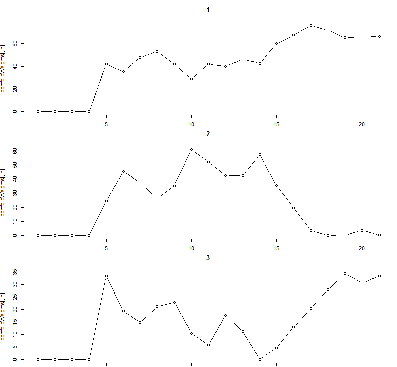
The above plot shows us clearly how the weights have changed for the sample systems within the whole back-testing period. Note that initially all weights are zero since there wasn’t any Markowitz optimization going on within the first 5 years. After this we can see how the weights start to change, notice how initially system 3 had a lot of weight, which started to decrease almost immediately as the Markowitz rolling window started to move. It is also worth noting that system 3 descended to an almost 0% contribution near year 14 just at the same time as system 2 reached one of its highest contribution points. After this system 2 started to decrease while system 3 increased substantially until it reached a new contribution high near 35%. System one on the other hand has increased steadily and has changed little during the past few years. This tells us that the historical view of how different systems reduce variance has changed significantly. We can also see the results of an approximate back-test to see how our performance would have looked like. To do this we first remove all data before year 6 (as we didn’t have any applied weights there) and we then combine the portfolioXTS into a single column within a portfolioCombination xts object using a simple loop to add returns (note that rbind won’t work here because you’ll have duplicate dates).

–

portfolioXTS <- portfolioXTS[ index(portfolioXTS) > 
index(portfolioXTS[12*6]),]

portfolioCombination <- portfolioXTS[,1]

for (j in 1:length(systemListTest$systemFileNames)) {
portfolioCombination[j,1] = 0
sum = 0
for (i in 1:length(systemListTest$systemFileNames)) {
sum = sum + portfolioXTS[j,i]
}

portfolioCombination[j,1] <- sum
}

portfolioCombination[is.na(portfolioXTS)] <- 0

colnames(portfolioCombination)[1] <- "markowitz portfolio"
portfolioCombination[is.na(portfolioCombination)] <- 0

#corrgram(data.frame(portfolioXTS))

charts.RollingPerformance(portfolioCombination)
charts.PerformanceSummary(portfolioCombination, ylog=TRUE)

–

–

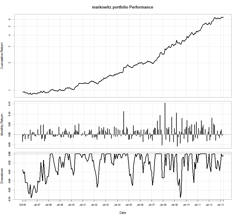
The above results show us how the portfolio did when switching between different system weights. As you can see the the maximum drawdown is around 9.6% while the additive drawdown for all systems is about 15%. We also have an increase in the annualized yearly return which is 11.6%, greater than that of the individual trading systems although clearly the final cumulative balance is not that high because we have 6 years less within the portfolio test. Interestingly the system does worst when it has to carry out switching as performance is compromised as the system weights get changed. For example when the contribution from system 2 changed to system 3 the portfolio showed some significant drawdowns.

This R script will allow you to test any rolling window Markowitz setup you want. My example uses a 5 year rolling window with yearly rebalancing but you can change the script to accommodate any rolling window or weight optimization frequency to see how this affects your systems. Clearly any Markowitz balancing scheme that worked well in the past might not work well in the future (because the way in which system correlations will change going forward is unknown) but you can certainly get an idea about how your portfolio responded to different management schemes in the past and how the ability of your different systems to reduce variance has changed through time.

If you would like to learn more about systematic trading and how you too can build your own highly linear systems for the creation of trading portfolios please consider joining Asirikuy.com, a website filled with educational videos, trading systems, development and a sound, honest and transparent approach towards automated trading in general . I hope you enjoyed this article ! :o)