The question of whether or not a financial time series follows a random walk is important as this determines whether or not you might be able to gain a statistical edge that is different from any inherent long term bias. This topic is often discussed across internet forums among retail traders, but you will not be able to find – at least I haven’t – any suggestion to use formal statistical tests in order to determine whether the market is actually random or not. This is quite surprising as there is a quite extensive array of statistical hypothesis tests in time series analysis that have been specifically designed to address the issue of whether or not a sample time series follows a random walk. On today’s post I am going to show you how you can use R to easily perform a powerful statistical test that will let you know whether or not the time series you’re analyzing is likely or not likely to be following a random walk. In particular we’re going to learn how to perform the test described by Lobato et al within this paper.
–
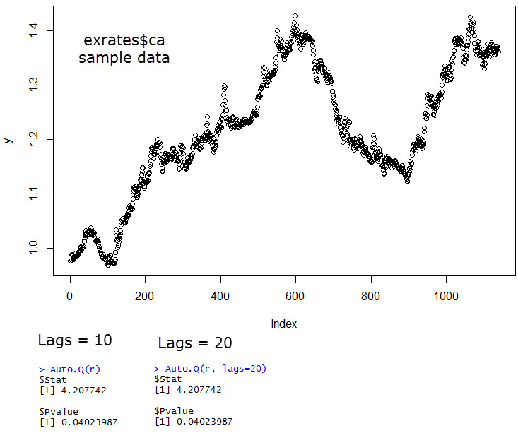
library(vrtests)
data(exrates)
y <- exrates$ca
nob <- length(y)
r <- log(y[2:nob])-log(y[1:(nob-1)])
Auto.Q(r)
–
–
First of all let us talk a bit about random walks. A time series follows a random walk if the results of subsequent moves in the series are completely independent of any previous movements. This effectively means that any attempt at predicting the next outcome of the series using any type of regression analysis will be completely unsuccessful with increasing time as the uncorrelated nature of the series implies that there can be no predictive power from analyzing the past. In addition random walks have some well defined properties that allow you to estimate a range of possible movements – which is useful for predicting things such as volatility – and this is the basis of many econometric practices in current markets that assume financial instruments follow random walks. The famous Black-Scholes model and the practice of delta hedging depend significantly on the assumption of random walks.
How can we test if a financial instrument follows a random walk? Most statistical hypothesis tests used to evaluate if a series is a random walk are based on the assumption of auto-correlation in the random walk model. Since there is no auto-correlation within a random walk, if we find a significant auto-correlation then the probability that the series is a random walk will be diminished. One of the easiest, most powerful and most robust tests to do this is the test suggested by Lobato in the paper linked above. The paper describes a Portmanteau test that automatically selects the auto-correlation lag to test, something that is incredibly useful as it frees the researcher from having to test a wide variety of lag periods, as it is needed across other tests.
–
library(vrtests)
#here I used a csv with Date OHLC columns
dataset <- read.csv("PathToData.csv") #replace with the absolute path to your csv
y <- dataset$Close
nob <- length(y)
r <- log(y[2:nob])-log(y[1:(nob-1)])
Auto.Q(r, lags=x) # replace x with the max lag you want (10, 20, 30, etc)
–
Many tests for random walks have been coded in the R package vrtests, which offers a variety of variance ratio tests plus many other useful tests for time series analysis. The test described by Lobato can be accessed through the Auto.Q function and contains only two parameters, the first is the return of the financial time series (log return) and the second is the maximum lag to be used by the test (the test will automatically choose a lag between 1 and this number). There are also some important considerations to be taken into account. Clearly a random walk may look none random with a higher probability as its length gets smaller (you could only tell with certainty if a series is a random walk if you had infinite data) so you should always keep in mind that the amount of data must be large (n>5000). It is also important to set the lags parameter to a value that is large enough as the default (10) is very low for financial time series, especially in time series belonging to intra-day periods, where auto-correlations are always going to be above the 1440/(timeframe in minutes) lag threshold (as phenomena like market opening times are cyclic in a daily manner).
–
–
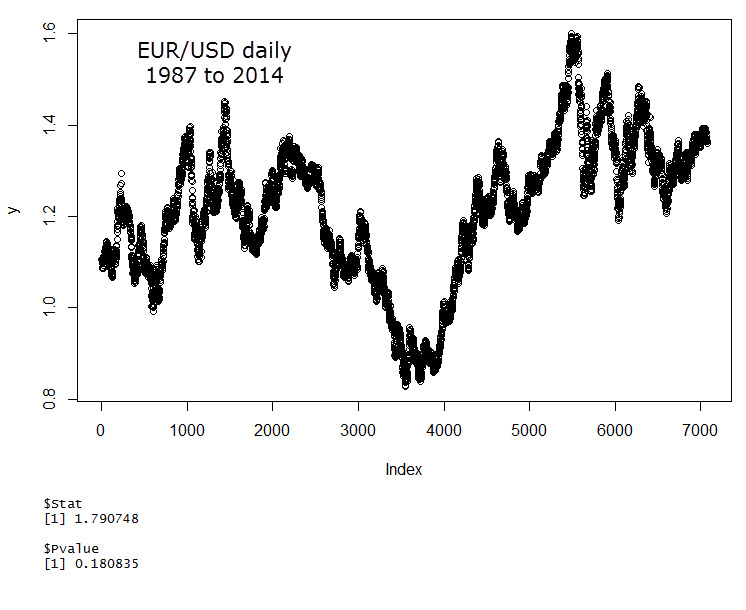
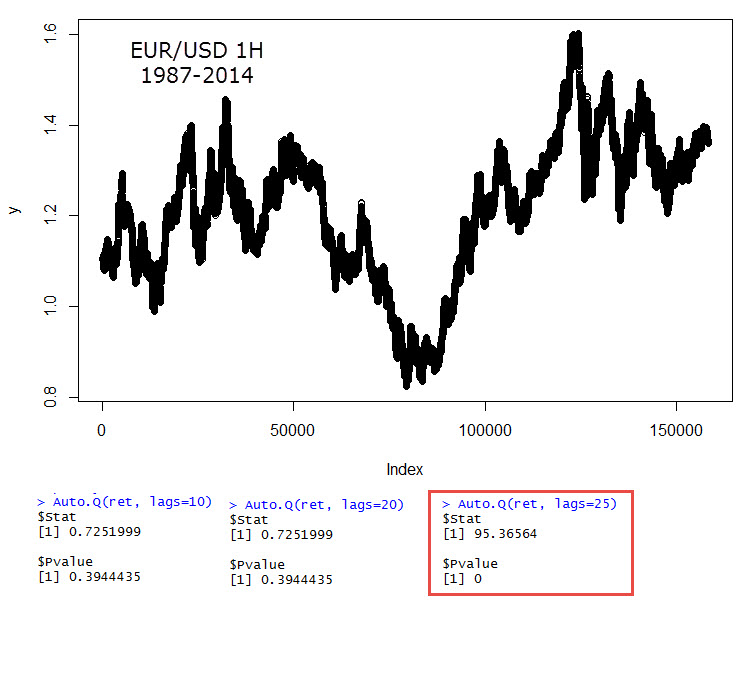
The code fragment showed above describes how to perform a simple example using the exrates$ca data available within R, containing about 1000 points of CAD/USD exchange rates. Since the data is daily you can see that the change in the p value with an increase in the maximum lag is non-existent. In this case the result of our test gives us a p-value of 0.04 which means that we can say above a 95% confidence that this data does not follow a random walk. I have repeated this experiment using EUR/USD daily data (1987-2014, 1987-1999 using DEM/USD) and obtained the results showed above (in this case the maximum lag also has no effect). In this case the p-value is 0.18 which means that we cannot say with enough confidence that this data does not follow a random walk. It is also interesting to use the EUR/USD 1H data (same time period) to see if this same phenomena happens across a shorter time frame. In this case it is obvious that auto-correlations are virtually non-existent with a max-lag below 25 but as soon as we get to this value (which is the lag expected for daily auto-correlations), our p-value drops below machine precision, such that the 1H can be said not to follow a random walk with a confidence above 95%. When running these tests it is useful to set the lags parameter (the maximum lag) to a large value as the test is able to choose the precisely needed value automatically, you will want to set lags to at least 2*1440/(timeframe in minutes). For timeframes at or above the daily, the default lags=10 seems to be enough.
Hopefully the above has showed you how you can easily carry out your own tests of the random walk hypothesis using the Portmanteau test suggested by Lobato et al. With this tool you no longer need to “guess” whether the markets are random or not but you can actually carry out a formal statistical procedure that will give you some evidence to support your case (no need for endless, argument-less ranting on internet forums). The above tests is quite robust and suitable for financial time series but I strongly suggest you read the entire Lobato paper if you’re interested in the test’s limitations and how it compares to other tests for the random walk hypothesis. If you would like to learn more about using R in trading please consider joining Asirikuy.com, a website filled with educational videos, trading systems, development and a sound, honest and transparent approach towards automated trading in general . I hope you enjoyed this article ! :o)


hi Daniel
A most interesting study. It’s quite odd that this topic is not much discussed in trading communities despite non-randomness being an essential prerequisite for successful trading.
Have you studied how the (non-)randomness trends through the years in an instrument (EURUSD, for example)? How about seasonality? Have you tried, for comparison, any non-forex instruments, the SPX for instance?
cheers
mikko
Hi Mikko,
Thanks for posting :o) Yes, I also find it quite surprising. However you should consider that randomness is indeed discussed very commonly across online retail trading communities but always in a very informal and speculative way with no use of statistical tools for the evaluation of the random walk hypothesis. To me this seems to make sense since while realizing that randomness is important is quite easy, knowing how to test for it is significantly harder. Perhaps this lack of insight into formal tools is just a consequence of a general lack of statistical knowledge from retail traders.
It would definitely be interesting to calculate something like a randomness indicator with the value of the Lobato test statistic for the past X bars, you will probably need X to be very large (at least 5000) so this might only be suited to the lower timeframes. However I haven’t done this yet, but it’s a nice idea to try. This should also give some insight into any possible seasonality in autocorrelations.
Yes, I have tried several equity ETFs on the daily TF, all of them so far can be described by using a random walk with drift model. Essentially equity markets are quite efficient but they do have a positive long term bias, therefore the best idea in equity markets – at least on the upper time frames – seems to be to use strategies that take advantage of this bias (momentum like strategies). In essence you’re better off attempting to maximize your ability to profit from the drift component. That said, my research in this area is still very preliminary and my lack of low TF information means that I am also unable to make deeper insights.
I hope this answers your questions. Thanks again for posting :o)
Best Regards,
Daniel
hi Daniel
Thanks for responding. Thought about this stuff a little more – the insight presented in your article is simple yet also very profound at the same time: making a wholesale claim that a market, any market, is efficient or not efficient is in most cases almost pointless unless a specific “lens” (timeframe) through which is observed is also specified. The proponents of the efficient markets hypothesis are directionally correct, yet the folks who don’t subscribe to that idea can also be right. It depends on what perspective you take and how exactly you define the scope of observation. Perhaps not such big news for market experts but for us regular people (and certain academics!) this is of substantial interest.
Just to check I understood correctly – your preliminary findings suggest that, broadly speaking, marketing timing methods applied to equity markets on daily and above timeframes generate no alpha? I suppose that this does not necessarily imply that timing as applied to individual constituents of said indices is useless too? You mention momentum strategies, but aren’t momentum approaches a form of timing strategy too? Therefore, provided that the random walk hypothesis (with drift) holds, they cannot produce alpha? They can still generate decent returns thanks to the inherent drift of course but not excess
cheers
mikko
Hi Mikko,
Thanks for your reply :o)
This is perhaps too broad, I would say that for the instruments I have studied you cannot be certain enough that you have alpha on these timeframes. Perhaps you could have alpha but the probability that you do not have it is high.
Sure, it does not imply that the answer is the same for individual stock components. You would have to carry out an analysis for each one to be sure.
Not necessarily. There are many different equity instruments (different market ETFs for example), all with different drift components that can and do change as a function of time. If you cannot obtain alpha from equities on the daily time frames you can still choose to follow the instrument that contains the largest drift component. Consider that there are mathematically optimum ways to trade combinations of random walk plus drift instruments. In this sense you don’t benefit from timing any individual component but you benefit from choosing the instrument with the highest prevailing drift. This is the sort of thing that ETF rotations attempt to do.
Of course, the long term bias in equities allows you to profit from the positive sum game character of the equity market, not from any alpha. There is also nothing forbidding you to profit from the markets with the highest drift component. As I mentioned before, if the indexes being traded all follow random walks with drift – especially a dynamic yet always positive drift component – then there is a mathematically optimum way to trade a combination of them.
I hope this better answers your questions :o) Thanks again for commenting,
Best Regards,
Daniel
Thanks for the comprehensive answer, Daniel. I’m not seeking to engage you in any sort of tutoring session but I find the topic very interesting, certainly in light of the impressive backtested results achieved by many ETF rotation schemes. Now trying to reconcile in my mind that apparent success with your findings of high likelihood of randomness. Intuitively it feels acceptable that one is able to find a market that has a strong trend / high momentum / high positive drift at a point in time. However if those markets indeed follow a random walk (with drift) then one would assume that the periods of high drift are randomly distributed too and therefore cannot be timed successfully, rendering momentum / rotation strategies ineffective (probably positive in the long term but devoid of any alpha).
What is the hole in my logic? Or can it be shown that genuine inefficiencies can be found in (ETF) markets, despite them having virtually zero autocorrelation, provided that time lag is appropriately chosen as per your reasoning with respect to 1HR TF in FX?
best regards
mikko
Hi Mikko,
Thanks for posting. I would argue that ETF rotations do not seek any alpha, they are merely ways of getting the best market performance from the bias component (results from the best drift component), you’re just attempting to always trade what is best. If you model different instruments with dynamic random walks with drift (for example an always positive, yet sinusoidal, oscillating drift) you’ll notice that you can trade them this way successfully. Sometimes you do in fact get into upward movements that are a larger consequence of the random walk component than the drift (where you take loses) but you often get into the components with the highest drift and make money. Rotations will never work on instruments that all follow simple random walks, but the drift component makes the rotations work. As the drift is non-constant, moving to what seems to be giving the highest drift will work in the long run.
As I said before, there are many ways to trade random walks with drift, rotations are just one of them and they do not constitute the obtaining of alpha (anything that is obtainable beyond the simple drift component). If you’re interested in this topic I would suggest the building of sample series in R (random walks with dynamic or static drifts) and the testing of different rotation schemes with them. You’ll see that they hold significant resemblance to what we obtain in global ETF rotations, you are able to obtain a performance that is superior to the best “single instrument” buy-and-hold trade. I think the results will answer a lot of the questions you might have.
Note that I am not saying that ETFs all follow random walks (I just have very preliminary results) but I’m saying simply that this is not needed for a successful ETF rotation strategy (As you can show by building a rotation model over a set of random walk + drift series). Thanks again for writing :o)
Best Regards,
Daniel
Hello,
I have tried library(vrtest) and library(vrtests) and Rstudio and R show “Error in library(vrtest) : there is no package called ‘vrtest’”. Has the package name changed?
Any suggestions?
Thanks
Tayo
Hi Tayo,
Thanks for writing. Try installing the library first install.packages(“vrtest”). Let me know if this helps,
Best Regards,
Daniel