During this month I showed you some preliminary successful results I obtained through the use of random forest classification algorithms for the prediction of out-of-sample performance using in-sample derived statistics. We saw how the models built in R compared to the models developed in python and we saw some of the rates of success I was able to initially obtain. Today we are going to go a bit further into the improvement of these classification algorithms, I will discuss some of the refinements I have made and will show you some of the accuracy and improvements in profitability I have got from these models. I will go through some of the observations I made and some analysis I performed to be able to take these classification efforts to the next level.
–

–
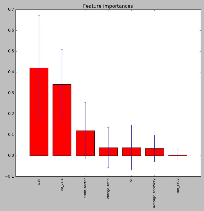
The idea of this classification exercise is to try to get an additional edge by predicting which models will fail and which ones will succeed during the first six months of live trading after the systems have been mined and validated. For this I have been using random forest classifiers which have been the only ones to show some degree of success. At first I used 28 in-sample statistical variables – back-testing statistics and system characteristics – but the random forest variable importance measurements soon revealed that this number was too high and most of these variables were always discarded. The image above shows the final variable makeup I have decided to use, these includes all the variables that gave an importance measurement above 0.01. As you can see we have the pair, number of break-even bars for the trailing stop mechanism, the profit factor, SL, mar ratio, omega ratio and average drawdown recovery length.
Interestingly the most important variable is the pair, which makes sense as different pairs show different behaviors and therefore correlations between IS/OS success might be different depending on which pair we are trading. Notice also that most of the in-sample statistics that ended up in the model are variables that are related to both profit and risk. The omega, mar ratios and profit factor are all risk adjusted return variables. The only one which is not from this family – the average recovery – is also intuitively important since systems with much slower recoveries will have a lower likelihood of being profitable after 6 months of trading. It is also worth noting that there are no linear correlations between any of these variables and the six month out of sample return, meaning that any relationships found are non-linear.
–

–
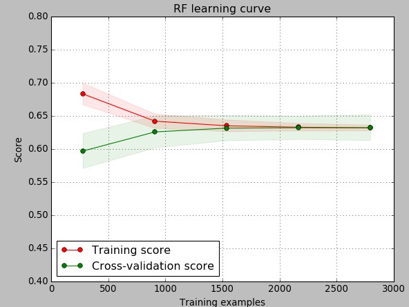
The next thing I wanted to take a look into is how the training/cross-validation errors change as a function of the training sample. For this I created a learning curve keeping 20% of the training set for cross-validation and using 20 model generation iterations to generate each point. As you can see the behavior we can observe is typical of complex problems, where the training error increases as a function of the number of samples while the cross-validation error decreases. We also see how both errors converge and in the end the actual variance of the problem is minimal with both the testing and training errors converging to almost the exact same average accuracy number. It is however true that overall model variance is higher in the testing sets – you can see that the shaded area showing the range of obtained accuracy values is larger – but overall we are always able to classify more than 60% of systems correctly. The above also shows why more than 1000 examples are needed, otherwise cross-validation errors are too high.
I did not perform any extensive optimizations of the random forest variables as they yielded no important improvements in the cross-validation prediction scores. The only variable I changed was the maximum depth – as the default is too large and generates a lot of overfitting – and I changed the number of estimators to 150 in order to reduce model variance to what you see above. Going to a completely independent validation set – which contains strategies that have yet to reach 6 months of trading but have more than 5 months – I obtained similar classification scores with an average value of 64% when averaging predictions over 6 generated random forest models, which is the same thing I obtained when doing the regular training/cross-validation within the original set. This is encouraging as it points to the achievement of some generalization by this classification methodology.
–

–
The above method always yielded a very significant improvement in the expected OS return in the validation set. The average out of sample return improved by 80-120% in relative terms, meaning that while the average daily return was negative for this validation set when trading all systems it turned positive when trading only systems that were classified to perform profitably within the 6 month interval after mining. In the next post of this series we will talk further about how this will be implemented in our live trading process and how we will improve the model going forward. If you would like to learn more about building models and how you too can trade large system portfolios please consider joining Asirikuy.com, a website filled with educational videos, trading systems, development and a sound, honest and transparent approach towards automated trading.strategies.


