In the past I’ve written some posts about system correlations and how measuring the historical correlation between trading strategies is fundamental to achieve the highest possible diversification when trading a portfolio. However in the past I gave some wrong (or perhaps only confusing) notions of rolling window correlations, which I will clear up within this post. Today we are going to look back at the use of rolling window correlations in order to make system-pairing choices, such that the amount of overall correlation between our strategies is minimized. We will be looking at the effect of the rolling window size as well as the practical implementation of this analysis using the quantmod, performanceAnalytics and the ggplot2 R libraries. After reading this post you should be able to carry out your own rolling window correlation analysis in order to decide which systems work best together in portfolios and which ones do not.
–
–
System correlations are important because they tell us how closely the returns of our trading strategies matched in the past. Given two trading systems A and B, the historical correlation between these systems determines how well their profit/drawdown phases paired. If A and B are both systems with long term historical profitability then we expect their overall balance correlation to be positive, because they are both growing balance curves and therefore they must have some matching between their returns as a function of time (their positive returns must inevitably match at some point since they both have more profit than loss). It is therefore essential to look at a rolling window correlation values in order to get an idea about the shorter term correlations between our trading systems. The larger our values, the more positive our correlations will become, provided both systems have similar overall profit values.
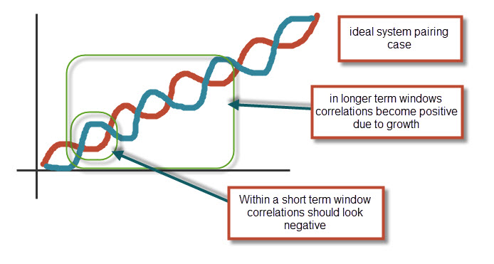
When looking at short term rolling window correlations, it is important to determine what the ideal scenario would be. In very short term window correlations a negative value would be ideal, since it would mean that our trading systems are completely decoupled from one another (see image above). This value may become more positive as the rolling window grows very large and the positive return character becomes inevitably correlated. Nonetheless we should expect two systems with good pairing to still have uncorrelated returns at significantly large windows (1000 days). It is therefore important to look at rolling window correlations on small windows and then select system pairing for which the correlation values are the smallest. Looking at varying window sizes should also give us some idea about the pairing behavior between our two strategies.
–
library(zoo)
library(quantmod)
library(PerformanceAnalytics)
library(ggplot2)

resultsTEMP <- read.zoo("E:/R_Experiments/25-01-2014/results.csv"
, sep = ",",format="%d/%m/%Y %H:%M", header=TRUE,index.column=1,
colClasses=c("character", "numeric"))
results<- as.xts(resultsTEMP)
dailyResults1 <- dailyReturn(results)

resultsTEMP <- read.zoo("E:/R_Experiments/25-01-2014/results2.csv",
sep = ",",format="%d/%m/%Y %H:%M", header=TRUE,index.column=1,
colClasses=c("character", "numeric"))
results<- as.xts(resultsTEMP)
dailyResults2 <- dailyReturn(results)

resultsTEMP <- read.zoo("E:/R_Experiments/25-01-2014/results3.csv",
sep = ",",format="%d/%m/%Y %H:%M", header=TRUE,index.column=1,
colClasses=c("character", "numeric"))
results<- as.xts(resultsTEMP)
dailyResults3 <- dailyReturn(results)

portfolio <- merge(dailyResults1, dailyResults2, dailyResults3)

portfolio[is.na(portfolio)] <- 0

colnames(portfolio)<-c("system1", "system2", "system3")

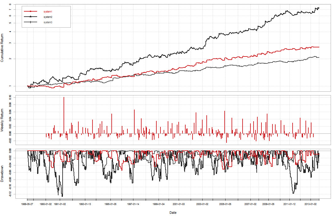
charts.PerformanceSummary(portfolio, colorset=redfocus, ylog=TRUE)
–
–
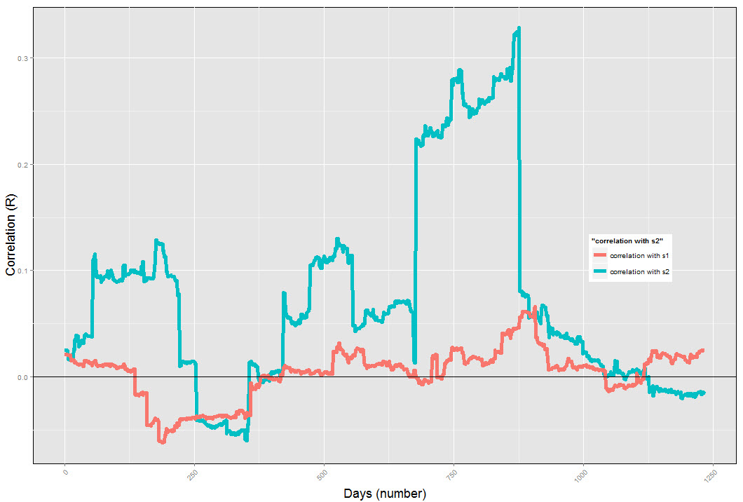
Let us now look at a practical example, we have 3 systems that we want to combine into a 2 system trading portfolio. We know from the start that we want to include system 3 due to its return to risk characteristics but we can only combine it with an additional system due to capital constraints (we don’t have enough capital to trade the 3 systems). We therefore have to make a choice between the system1-system3 and the system2-system3 pairing. Making this choice based entirely on the profit curves would be sub-optimal, since the objective of our portfolio building exercise is to use the system combination that can minimize our risk the most by making correlations as small as possible. The code above generates the performance graph for all of our trading systems. As you can see both systems 1 and 2 have a highly linear behavior in the logarithmic domain and it is not clear which one of these strategies might combine better with system 3. We can now use the quantmod library to perform a rolling window correlation analysis (we define delcor31 and delcor32 as the 200 day rolling window correlations of system3 returns with system1 and system2 returns respectively). We then use ggplot2 to generate some pretty graphics.
–
delcor32 <- runCor(portfolio$system3, portfolio$system2, n=200,
use="all.obs", sample=TRUE, cumulative=FALSE)
delcor31 <- runCor(portfolio$system3, portfolio$system1, n=200,
use="all.obs", sample=TRUE, cumulative=FALSE)
correlations <- merge(delcor32, delcor31)

correlations <- na.omit(correlations)

p <-ggplot(correlations, aes(x=index(delcor32)))
p <- p + geom_line(size=2, aes(y=delcor32, colour="correlation with s2"))
p <- p + geom_line(size=2, aes(y=delcor31, colour="correlation with s1"))
p <- p + ylab("Correlation (R)")
p <- p + xlab("Days (number)")
p <- p + theme(axis.title.y = element_text(size = rel(1.5)))
p <- p + theme(axis.title.x = element_text(size = rel(1.5)))
p <- p + theme(axis.text.x = element_text(angle = 45, hjust = 1))
p <- p + theme(panel.background = element_rect(colour = "black"))
p <- p + geom_abline(intercept = 0, slope = 0)
p <- p + opts(legend.position = c(0.85, 0.45))
p
–
–
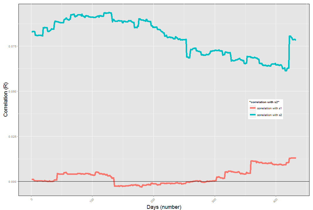
As you can see on the image above, the rolling window correlation shows us that system 2 is not an ideal pairing with system 3 because results in the short term are much more positively correlated than with system1. It is therefore ideal to avoid pairing system 2 with system 3, because our drawdown periods are bound to be deeper due to the inherent correlation between these two strategies in short term windows. System 2 will most likely be unable to increase the linearity of the System 3 returns in the logarithmic scale (smooth results) as much as system 1 will. It is also interesting to look at longer term (say 500 day) rolling window correlations. We can see here that system 1 is still able to maintain a very low correlation with system 3 results while the correlation with system 2 is also smaller (sorry for the color inversion between systems relative to the last image). At 1000 days, the differences become even clearer and it is obvious that the correlation with system 2 is larger than with system 1. It is therefore easy to conclude that the best pairing here would be between system3 and system1 and not between system2 and system3.
–
–
By using system3 and system1 together we will be trading under the assumption that the correlation of returns remains practically at zero as time evolves. This means that the daily returns of these systems are almost completely uncorrelated, something that is beneficial to our trading setup. A good signal of portfolio failure would also be a significant increase in the correlation of returns between our systems, so monitoring the rolling window correlations as a function of time is also important in order to assess how good your system pairing stays as time goes by. If you would like to learn more about portfolio building and how you too can create a portfolio of algorithmic systems for live trading please consider joining Asirikuy.com, a website filled with educational videos, trading systems, development and a sound, honest and transparent approach towards automated trading in general . I hope you enjoyed this article ! :o)


