Mechanical Forex

Last week Bob – an avid and frequent reader – posted a comment with a suggestion involving the generation of random financial time series in order to generate an estimate for data mining bias within my system generator, Kantu. After carrying this analysis out – which will be posted this week as well – I searched for some information about the generation of random financial time series to compare my results to but I couldn’t find anything online outside of academic papers. Due to this reason I decided to write a blog post with a tutorial on the generation of random financial time series using R which I hope will be a useful starting point for anyone wishing to generate random financial time series data. Through the following paragraphs I am going to explain how I generated my random data, what I can do with it, what I cannot do with it and what steps or changes need to be implemented depending on the use that the random financial data is going to have.

First of all we should understand that there are many different potential uses for random financial time series (a.k.a synthetic data) and the intended use determines how we generate the data. Financial time series have several key features and the way in which we generate a synthetic series depends on which components of this data we want to reproduce. For example if you want to test a trading system on synthetic data to assess robustness you need to generate synthetic data that faithfully reproduces all overall statistical characteristics of the original time series while if you’re generating data for the testing of data mining bias (what I intended to do) you want data that is as close to a random walk as possible (make sure the data can only lead to spurious correlations). It is obviously very complicated to reproduce the statistical characteristics of a time series to do synthetic system testing (you would need to reproduce seasonality, serial correlations in volatility, etc) so this tutorial will cover only the most basic case, generating a time series that resembles a random walk. Note that there are many ways to do this and the tutorial below only highlights what I found to be the easiest. Before following this tutorial I would also advice you to read my previous two (1 , 2)R tutorials on basic time series analysis, so that you are familiarized with some basic R commands.

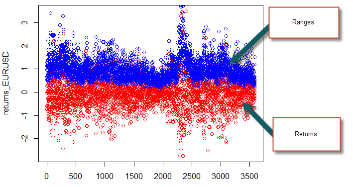
To start our generation of random data we first want to load a csv containing the time, open, high, low, close and volume variables for a sample time series (this can be any symbol). We’ll use this real time series to obtain some realistic measurements of standard deviations and means for our synthetic data. After we have loaded the data we then calculate two variables containing the return and ranges for the financial time series, as we did on the previous R tutorial. As I said before there might be an easier way to do this in R but this was the easiest way I could find (yes, I am guilty of looping, I cannot shake off the C++). We can also plot the range and the returns to see that we got things correctly.

–

dataset <- read.csv("C:/PathToData/EURUSD_1440.csv")
returns_EURUSD <- diff(dataset$Close)

for (i in 1:length(dataset$Close) ) {
returns_EURUSD[i-1] = 100*(dataset$Close[i]-dataset$Close[i-1])/dataset$Close[i-1]
}

range_EURUSD <- diff(dataset$Close)

for (i in 1:length(dataset$Close) ) {
range_EURUSD[i-1] = 100*(dataset$High[i]-dataset$Low[i])/dataset$Close[i-1]
}

plot(returns_EURUSD, col='red')
points(range_EURUSD, col='blue')

–

–

The following step is simply to generate normally distributed random returns and  distributed ranges so that we can use these new values to generate our synthetic data. While we use the mean and standard deviation from the real financial data to generate the random ranges we use a mean of zero and the standard deviation for the returns for the random returns  as we don’t want our random walk to have any sort of long term bias (which might be introduced by a non-zero mean). We also generate a random column between zero and one for each candle which will determine the position of the open within the trading range. Note that this methodology eliminates all the serial correlation in volatility, a feature of real financial time series that doesn’t necessarily need to be present within a random series (correct me if I’m wrong!). We can also obtain histograms and plots for our random returns and ranges to see how they look. Notice that they are very difference from the original ones, looking much more random. However the distributions are normal, as evidenced by the histograms.

–

dataset$RandomRangeOrigin <- runif(length(dataset$Close), 0, 1)

dataset$normalRandomReturns <- rnorm(length(dataset$Close), 
mean = 0, sd = sd(returns_EURUSD))

dataset$normalRandomRanges <- abs(rnorm(length(dataset$Close), 
mean = mean(range_EURUSD), sd = sd(range_EURUSD)))

plot(dataset$normalRandomReturns, col='red')
points(dataset$normalRandomRanges, col='blue')
hist(dataset$normalRandomReturns,breaks=60,col='grey')
hist(dataset$normalRandomRanges,breaks=60,col='grey')

–

–

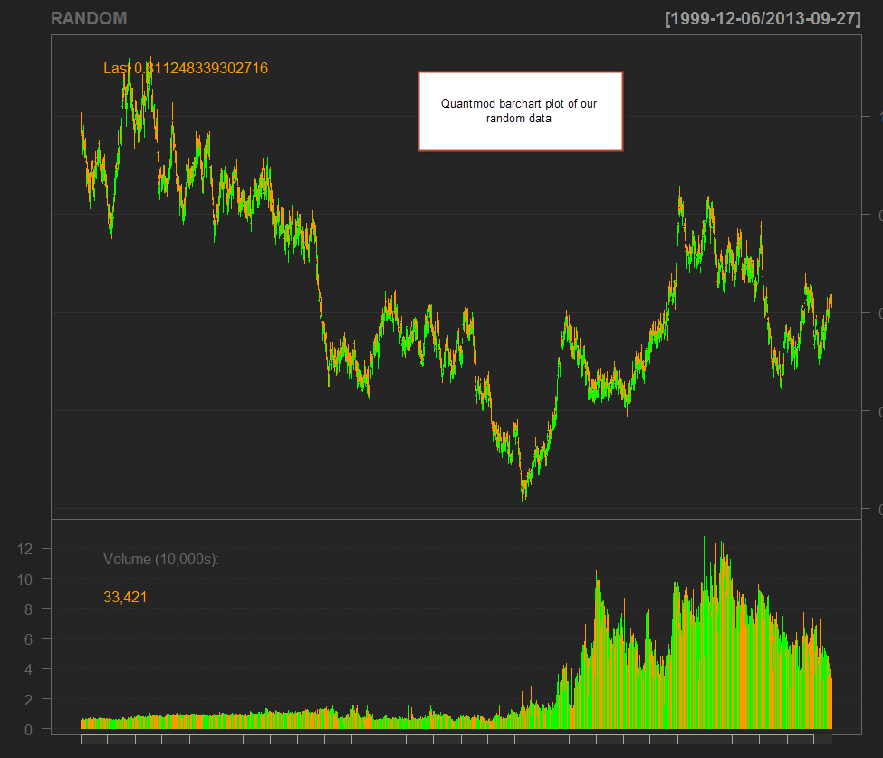
The final step is to use the above information to generate a synthetic financial time series. In order to do this we simple set the values for the first bar and then go through a loop that generated the new OHLC values using the randomly generated returns and ranges we have defined before. After doing this we then proceed to eliminate these columns (the random returns, ranges and origin) and we then save our data to a csv file. Note that the row.names=FALSE option is used in order to avoid saving of a numerical value on each row of the csv file. With the file saved we can then load the quantmod library (make sure you have it installed) and carry out a simple plot of our data using the barchart function after loading our CSV into an xts (you might need to change the date formatting on the read.zoo function if your csv is not in Y-M-d format (like 1990-12-23)). We will look into quantmod with more detail on a tutorial later on ;o).

–

dataset$Open[1] = 1

dataset$High[1] = dataset$Open[1]+0.01*(1-dataset$RandomRangeOrigin[1])
*dataset$normalRandomRanges[1]*dataset$Open[1]

dataset$Low[1] = dataset$Open[1]-0.01*dataset$RandomRangeOrigin[1]
*dataset$normalRandomRanges[1]*dataset$Open[1]

dataset$Close[1] = dataset$Open[1]+0.01*
dataset$normalRandomReturns[1]*dataset$Open[1]

for (i in 1:length(dataset$Close) ) {

if (i>1){
dataset$Open[i] = dataset$Close[i-1]

dataset$High[i] = dataset$Open[i]+0.01*(1-dataset$RandomRangeOrigin[i])*
dataset$normalRandomRanges[i]*dataset$Open[i]

dataset$Low[i] = dataset$Open[i]-0.01*dataset$RandomRangeOrigin[i]
*dataset$normalRandomRanges[i]*dataset$Open[i]

dataset$Close[i] = dataset$Open[i]+0.01*
dataset$normalRandomReturns[i]*dataset$Open[i]

}
}

dataset$normalRandomReturns <- NULL
dataset$normalRandomRanges <- NULL
dataset$RandomRangeOrigin <- NULL

write.csv(dataset, "C:/PathToData/RANDOM_DATA.csv", row.names=FALSE)

RANDOMtemp <- read.zoo("C:/PathToData/RANDOM_DATA.csv", 
sep = ",",format="%Y-%m-%d", header=TRUE,index.column=1,colClasses=
c("character",rep("numeric",5)))

RANDOM<- as.xts(RANDOMtemp)
head(RANDOM)
barChart(RANDOM)

–

–

With this tutorial you have been able to generate random financial time series data following the assumption of normally distributed returns and ranges with no serial autocorrelation (which should be perfectly market efficient). This random data should be useful to carry out measures such as data-mining bias, since no relationships within the data can lead to any profitability through anything except spurious correlations. You can use the CSV produced to load the data into other programs or use the xts to carry out any additional simulations using quantmod. Thanks a lot to Bob who inspired this post on random financial time series with his comments :o). If you would like to learn more about algorithmic trading and how you too can generate systems using algorithmic approaches please consider joining Asirikuy.com, a website filled with educational videos, trading systems, development and a sound, honest and transparent approach towards automated trading in general . I hope you enjoyed this article ! :o)