In the past we have explored the notion of how to know whether a system is or isn’t under-performing across a certain time span by looking at either fractions of historical performance (see this post) or Monte Carlo simulations (see this post). Another question besides whether a system is under-performing or not is when we can expect a system to behave at least as well as it behaved within our simulations. How much time should it take for a system to show statistics that are equal to those that we expect from out tests? On today’s post we are going to look at how we can answer this question using the qqpat library. We will see the difference the confidence intervals make in the estimation of the statistics and how long it’s bound to take us to achieve the long term CAGR and Sharpe values. You can download the code and sample system results here.
–
import pandas as pd
from pandas_datareader import data
import datetime
import csv
import matplotlib.pyplot as plt
import qqpatAsirikuy.com

def lastValue(x):
    try:
        reply = x[-1]
    except:
        reply = None
    return reply

system_list = ["sys0"]

for index, system in enumerate(system_list):
    tradeTimes = []
    tradeBalance = []
    with open(system + ".txt", 'rb') as csvfile:
        reader = csv.reader(csvfile)
        for idx_data, row in enumerate(reader):
            if idx_data > 0:
                tradeTimes.append(datetime.datetime.strptime(row[3], '%d/%m/%Y %H:%M'))
                tradeBalance.append(float(row[10]))
        if index == 0:
            data = pd.Series(data=tradeBalance, index=tradeTimes).resample('D', how=lastValue).pct_change(fill_method='pad').fillna(0)
        else:
            data = pd.concat([data, pd.Series(data=tradeBalance, index=tradeTimes).resample('D', how=lastValue).pct_change(fill_method='pad').fillna(0)], axis=1)

data = data.fillna(0.0)

analyzer = qqpat.Analizer(data, column_type='return', titles=system_list)
long_term_sharpe = analyzer.get_sharpe_ratio()[0]
long_term_cagr = analyzer.get_cagr()[0]
print long_term_sharpe
print long_term_cagr
sharpes90 = []
sharpes80 = []
sharpes70 = []
sharpes60 = []
cagr90 = []
cagr80 = []
cagr70 = []
cagr60 = []
periods = range(100,1000,100)

for i in periods:
    stats = analyzer.get_mc_statistics(index=0, iterations=1000, confidence=90, period_length=i)
    sharpes90.append(stats['wc_sharpe'])
    cagr90.append(stats['wc_cagr'])
    stats = analyzer.get_mc_statistics(index=0, iterations=1000, confidence=80, period_length=i)
    sharpes80.append(stats['wc_sharpe'])
    cagr80.append(stats['wc_cagr'])
    stats = analyzer.get_mc_statistics(index=0, iterations=1000, confidence=70, period_length=i)
    sharpes70.append(stats['wc_sharpe'])
    cagr70.append(stats['wc_cagr'])
    stats = analyzer.get_mc_statistics(index=0, iterations=1000, confidence=60, period_length=i)
    sharpes60.append(stats['wc_sharpe'])
    cagr60.append(stats['wc_cagr'])
    print i

fig, ax = plt.subplots(figsize=(12,8), dpi=100)
ax.set_xlabel('Period length (days)')
ax.set_ylabel('Sharpe')
ax.plot(periods, sharpes90)
ax.plot(periods, sharpes80)
ax.plot(periods, sharpes70)
ax.plot(periods, sharpes60)
ax.axhline(long_term_sharpe, linestyle='dashed', color='black', linewidth=1.5)
plt.show()

fig, ax = plt.subplots(figsize=(12,8), dpi=100)
ax.set_xlabel('Period length (days)')
ax.set_ylabel('CAGR')
ax.plot(periods, cagr90)
ax.plot(periods, cagr80)
ax.plot(periods, cagr70)
ax.plot(periods, cagr60)
ax.axhline(long_term_cagr, linestyle='dashed', color='black', linewidth=1.5)
plt.show()
–
When you start trading a system that has 30 year profitable back-test the expectation is for it to behave profitably right from the start. We often believe that if it has behaved well during 30 years it definitely should start behaving well right away and make money for us from the get-go. In reality we know that short term performance has a lot of inherent randomness and we know that it will take a significantly long amount of time before the statistics expected from long term performance start to show up. Monte carlo simulations – for systems where the assumptions made by the simulation are realistic – allow us to evaluate thousands of scenarios and measure the probability to achieve a given statistic within a certain confidence interval.
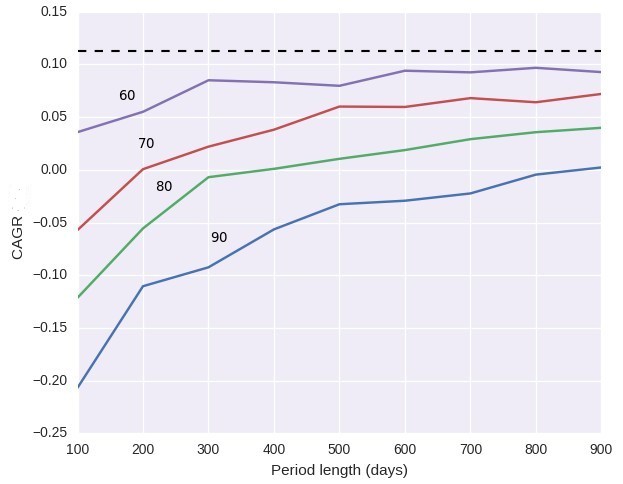
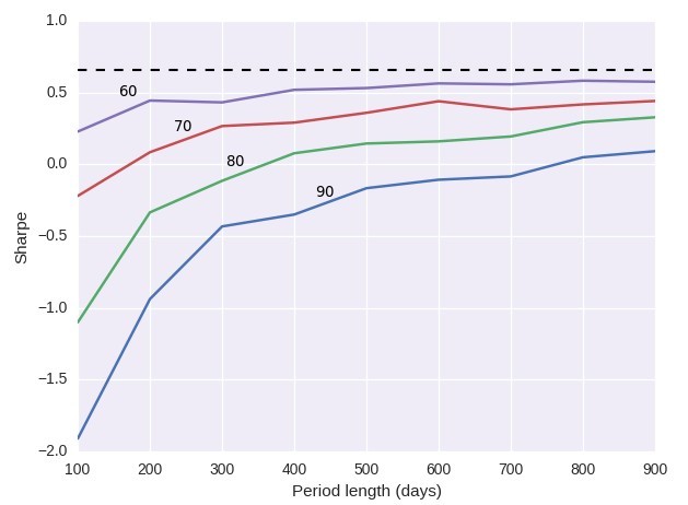
The code above performs Monte Carlo simulations for 4 different confidence intervals (60, 70, 80 and 90) and plots the Sharpe and CAGR values as a function of the simulation length for an included sample system, the graphs also include the long term Sharpe and CAGR values as doted horizontal lines. A 60% confidence means that we expect 60% of values to be better than this while a 90% confidence means that we expect 90% values to be better than this. This means that if, for example, the CAGR at 800 days at 60% confidence was 0.10 (10%) we would have a 60% probability to have a better value within our trading and a 40% probability to have a worse value. Since we want to have a probability above chance to see the statistic I didn’t include any confidence intervals at 50% or lower.
–
–
The graph above shows that achieving the long term CAGR is no easy feat. The long term CAGR was a measurement taken using 30 years of data and therefore it is only reasonable to expect that convergence towards the long term statistics will be slow. We can see that we immediately start with a higher than 50% probability to be positive – at only 100 days we already have a positive CAGR at a 60% confidence interval – but then the crawl towards the long term CAGR is really slow. At two years of trading we already have a good chance to be more than half-way there but there are other plausible scenarios that put us very far away. For example at a 90% confidence we could still be in slightly negative territory so our system could still be behaving within the distribution of returns given by the long term back-test and still be within a drawdown period. Only after more than three years of trading does the expectation at 90% confidence become positive and we’re not even close to the long term statistical value.
The Sharpe ratio curve showed below follows a similar behavior. We start with a high probability of being on the profitable side but it still takes long to reach even close to the long term Sharpe with a significant probability to be even much lower. As in the case of the CAGR at 90% confidence the Sharpe only becomes positive after around 3 years of trading. Notice that although we have a 60% probability to start better than 0.0 at 100 days we could still start at -2.0 and this still would be within what the system can give us. It would actually take around 10 years for the 90% Sharpe to be close to the long term Sharpe from the simulations, this is expected since the long term Sharpe took 30 years to be calculated and therefore we should approach that value if we really want to get close to the value of the original return series.
–
–
This is a reality that is disappointing to many. The nature of trading implies a relatively high uncertainty in the short term that may imply substantially probable and long periods of loss before important profits are realized. Sadly this is the nature of sustainable speculative trading, edges are based on the expression of long term bets on specific event types with a positive expectancy that will only show after a long amount of time. Trading strategies in financial markets is like trying to obtain a net additional amount of heads or tails from a slightly biased coin. In the short term the results may even strongly contradict those expected from the coin’s bias (in the short term you might have 10 consecutive tails on a slightly biased contain towards heads) but after thousands of trials it will becomes obvious that the coin is biased as expected. This of course makes trading hard and the eagerness to attempt to cheat this process – with often disastrous results common (as you can see here) – really high. You can only get a high chance of short term success if you have a certainty of long term failure.
Of course if you have a high probability to start with the right foot then the best thing you can do is to have as many systems as you possibly can to ensure that the overall likelihood of good results across shorter period is higher. The above issues still remain true but they are alleviated – volatility is reduced and the likelihood of positive results becomes higher – as the number of systems increases. If you would like please consider joining Asirikuy.com, a website filled with educational videos, trading systems, development and a sound, honest and transparent approach towards automated trading.