Mechanical Forex

Diversification is a very important force in algorithmic trading. Most systematic traders will not put all their resources under the management of one strategy but will attempt to diminish risk by diversifying their bets between different historically successful trading systems. After you gather several strategy candidates for live trading the question then becomes how to weight these strategies in order to come up with the combination that gives you the best result. But how do you do this? How do you calculate the weights for your different strategies? Do you maximize historical profits? Do you minimize risk? The answers to these questions are given by Markowitz portfolio theory which we can use to derive weights for our trading strategies. On today’s post we are going to learn how we can use this powerful tool in order to create balanced portfolios that give us the best compromise between risk minimization and profit maximization. As always, I recommend you use R studio for the application of this tutorial. The csv data for the back-tests used for this post can be downloaded here as well.

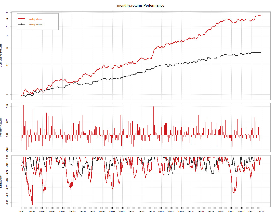
The first thing you will want to do is run compounding simulations for all your trading strategies and place their results into csv files with 2 columns, the first with your trade closing dates and the second one with the balance change for each trade. Please look into the zip file linked above for two examples showing the format I’m using for this tutorial (you can use other formats but you’ll have to modify the R code for the loading of the csv files into XTS objects).  After you have this done make sure you have the xts, fPortfolio, PerformanceAnalytics and quantmod libraries installed within your R setup so that you can execute all the code below. In order to combine systems in R we are first going to load our results into xts files and use the monthlyReturn function from quantmod in order to get monthly return values. We then merge these values into a single object, replace any NA occurences with zero and plot our two system summaries to check that everything went ok.  In this case I’ll be doing this for 2 systems but you can do this for as many systems as you want by appropriately modifying the code.  Note that I’ve plotted the system summaries along a logarithmic axis to make things easier to interpret.

–

library(xts)
library(quantmod)
library(fPortfolio)
library(PerformanceAnalytics)

resultsTEMP <- read.zoo("C:/PathToCSV/results.csv", 
sep = ",",format="%d/%m/%Y %H:%M", header=TRUE,index.column=1,
colClasses=c("character",rep("numeric",1)))

results<- as.xts(resultsTEMP)

monthlyResults1 <-monthlyReturn(results)

resultsTEMP <- read.zoo("C:/PathToCSV/results2.csv",
 sep = ",",format="%d/%m/%Y %H:%M", header=TRUE,index.column=1,
colClasses=c("character",rep("numeric",1)))

results<- as.xts(resultsTEMP)

monthlyResults2 <-monthlyReturn(results)

portfolioXTS <- merge(to.monthly(monthlyResults1, indexAt="firstof",
 OHLC=FALSE), to.monthly(monthlyResults2, indexAt="firstof", 
OHLC=FALSE), all = TRUE)

portfolioXTS[is.na(portfolioXTS)] <- 0

charts.PerformanceSummary(portfolioXTS, colorset=redfocus, 
ylog=TRUE)

–

–

Once we have our merged data loaded into the portfolioXTS object we must now convert this to a regular timeSeries object so that we can use the fPortfolio functions used to construct the portfolio object. We can do this by using the as.timeSeries function. After this we then change the names of the columns to “system1” and “system2” to make the portfolio results we’re going to get a bit easier to interpret. There are several different functions we can use to obtain our portfolio weights, we can maximize profits, minimize risk, minimize variance or maximize efficiency (risk and profit compromise). For this example we are going to obtain portfolio weights in which we minimize the variance of the resulting portfolio. You can look at the fPortfolio pdf manual for more information regarding the functions available for the calculation of portfolio weights. Notice how we use the “long only” constraint for the creation of the portfolio, this does not mean that we are using only “long positions” but that the data is combined “as is”. Since the fPortfolio library was designed initially to combine equity returns, the availability of shorting allows the portfolio to combine the inverse of some series (something we don’t want since we are combining systems).

–

resultsTimeSeries <- as.timeSeries(portfolioXTS)
colnames(resultsTimeSeries)<-c("system1", "system2")
minvariancePortfolio(resultsTimeSeries, constraints = "LongOnly")

–

–

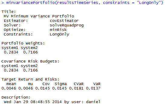
With these results we now have the optimum portfolio weights to use in order to obtain the least possible variance within our portfolio. Additionally the results show us the estimated mean, mu, covariance, sigma, CVar and VaR for our monthly returns. With this you now know that if you combine system1 and system2 in 0.2834 and 0.7166 weights, you are bound to obtain a portfolio with a mean monthly return of 0.46% with a variance of 1.3%. We can also look at the frontier plots for this portfolio in order to see which other risk/return values would be possible using different combinations of system1 and system2. You can easily do this using the fPortfolio library by creating a frontier object using your portfolio object and then using the plot function to create the frontier plot and add several different points of interest.

–

frontier = portfolioFrontier(resultsTimeSeries,constraints = "LongOnly")
plot(frontier)

–

–

The above plot reveals that for only a little additional variance we can obtain a significantly higher profit level (the most efficient portfolio, which is the tangency portfolio). However it is worth mentioning that any fitting of the portfolio towards an efficient frontier carries with it a fundamental assumption regarding historical correlations. The best way of combining portfolios with the least chance of being disappointed is to attempt to minimize variance as we did above. Although the profit might not be the historical best from the combination given, it’s more important to minimize risk when there is a general uncertainty about the future correlation between the systems used.

By following the above tutorial you should have been able to carry out a simple optimization of portfolio weights in order to find those that give you the least risk. Furthermore, the efficient frontier plots allow you to see the improvement in risk/profit measures for your portfolio as the two systems are combined in different fractions. Within a future post we will learn how we can also obtain simulation results for a system portfolio combination so that we can see the actual profit and drawdown characteristics that are generated after we apply our optimized portfolio weights. If you would like to learn more about portfolio trading and how you too can generate a set of algorithmically generated strategies for live trading please consider joining Asirikuy.com, a website filled with educational videos, trading systems, development and a sound, honest and transparent approach towards automated trading in general . I hope you enjoyed this article ! :o)