On a recent blog post I wrote about a new input/output structure for machine learning algorithms where the outputs are multiple potential trading outcomes using different types of trade management techniques (in that case different initial stop values). On that post I went over some of the basic notions of this technique and why it may prove to be a better solution compared to the single outcome outputs we’re using at this point within the Asirikuy community. On today’s article I will go a bit deeper into the practical problems when using these algorithms and some initial results using them on the EUR/USD. I will tell you about some of the decisions that have to be made when deciding to use these setups as well as how the overall optimization process changes.
–

–
Many things change when we move from single outcome to multiple trade outcome predictions. While with single outcome predictions we get two outputs – one predicting the outcome of a long trade and another the outcome of a short trade – when we go to multiple outcome predictions we now get 2 times N outcomes where N is the number of different trade management methods we want to predict. Given the increase in the output array complexity we get a change in the optimum machine learning parameters needed to predict these variables successfully through the back-testing process.
The two main machine learning variables used within our general system creation process are the number of inputs used and the number of examples used to train the machine learning algorithm on each bar (remember that our algorithms are constantly retrained using a moving window of examples through the back-testing process). When the number of outputs is increased the optimum values for these variables change – because you simply don’t need the same inputs or examples to properly train for 2 or 20 variables – often meaning that we need to trade using more inputs and using more examples to get to the best possible result for the machine learning algorithm. The advantage is of course that we eliminate the need to include an SL and other trade management parameters within the system so our overall number of needed tests per optimization drops exponentially. Since the ML running time increases less than what is gained from eliminating this additional parameters we obtain a net improvement in the total time needed to perform the optimization process.
–

–
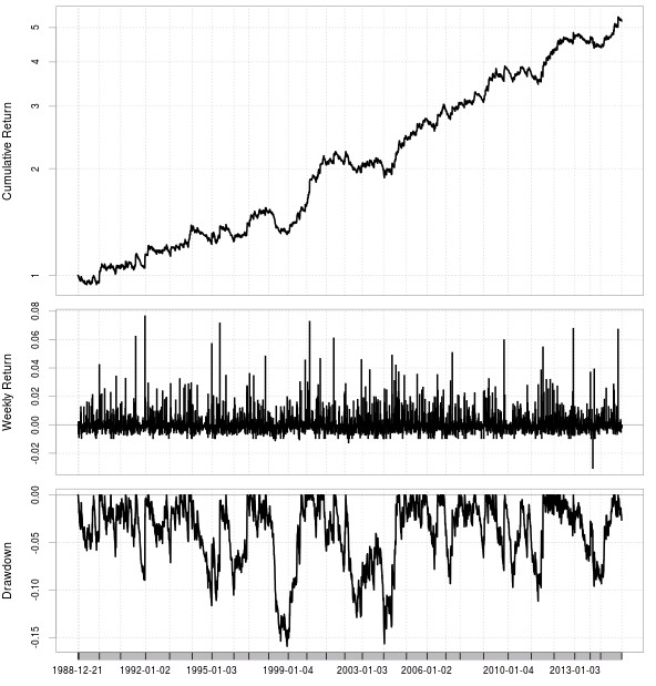
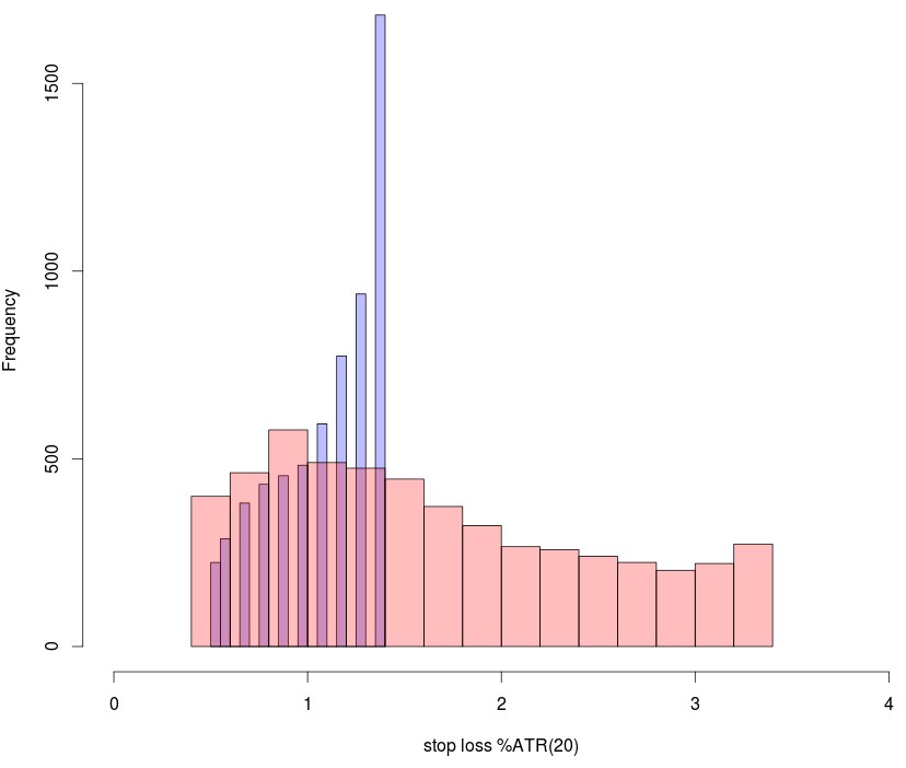
Another relevant question is how many trade outcomes you would need to include. In my initial experiments using the SL as the only trade management parameter I looked at the results of using 10 or 30 different trade outcomes which means exploring SL values from 0.5 to 1.5 or from 0.5 to 3.5. After obtaining two highly linear examples for both cases (highly linear system for the 30 outcome case is the first image on this post) through optimizations of the machine learning variables showed above I then created the SL histogram showing the SL selection of the ML algorithms for the two cases. As you can see in the case of the algorithm that goes from 0.5 to 1.5 there is a strong increase of frequency towards the 1.4-1.5 classes while in the case of the 0.5 to 3.5 algorithm there is a much smoother distribution of the SL values with the frequency reaching a maximum close to 1 and then dropping constantly up to the end at 3.5. There is however a slight increase at the highest value which points to a “border effect” at the highest SL value. This border effect is much more pronounced when a limited number of outcomes is used compared to when a wider range is present.
Interestingly if you take the parameters of the 10 outcome experiment and use it on the 30 outcome experiment you get a similar frequency increase on the last point of the frequency distribution, pointing to the fact that this border effect may also be related with the specific values of the ML parameters used to trade the algorithms. This effect is especially prominent when the frontier used to examine trade outcomes is large, pointing that large frontiers favor the limit cases of the SL because this achieve the highest potential gain in absolute terms a significant percentage of the time.
–

–
This points out to another vital issue when using multiple trading outcomes which is how to decide what specific outcome to trade. In the above example I first filtered outcome predictions to only take into account those that are “well behaved” this means those where the short trade outcome was greater than zero and the long trade outcome lower than zero or vice versa, meaning that the prediction in general makes sense. After this I then chose the outcome for which the short to long difference was the highest and entered a trade in the direction of the predicted positive value, with the trade being managed as instructed by that particular trade outcome’s logic. However this way of selecting creates a favoring of larger stop vales on larger frontiers, which can potentially be solved by using the largest ratio (short/long) instead of simply the difference.
As you can see we are only stratching the surface of the possibilities and the complexities inherent to this multiple outcome based machine learning. In time we will learn more and be able to draw better implementations that can overcome some of the important issues mentioned above. If you would like to learn more about building machine learning systems and how you too can code your own constantly retraining strategies please consider joining Asirikuy.com, a website filled with educational videos, trading systems, development and a sound, honest and transparent approach towards automated trading.


