Last time on the “Using OpenKantu in practice” series we learned how to use the free and open source OpenKantu software to evaluate the pseudo out of sample results of high winning ratio, almost never-losing strategies. Today we are going to see how we can evaluate the deterioration of systems in a pseudo out-of-sample period using OpenKantu and the R statistical analysis software. For this tutorial you will need to have OpenKantu installed as well as R with the ggplot2 package. I also recommend you install the R Studio software which makes using the R language much easier. After going through this post you will be able to run a simply analysis that will show you how much systems are expected to deteriorate in a pseudo out of sample according to the in-sample mining method you have used.
–
library(ggplot2)
data <- read.csv("/home/daniel/openkantu_data.csv")
data$P <- NULL
data$No. <- NULL
data$Symbol <- NULL

p <-ggplot()
p <- p + geom_point(size=3, aes(x=data$Profit.trade ,y=100*(data$OSP.trade-data$Profit.trade)/data$Profit.trade))
p <- p + ylab("Change in Profit per trade (%)")
p <- p + xlab("IS Profit/Trade (USD)")
p <- p + theme(axis.title.y = element_text(size = rel(1.5)))
p <- p + theme(axis.title.x = element_text(size = rel(1.5)))
p <- p + theme(axis.text.x = element_text(angle = 45, hjust = 1))
p <- p + theme(panel.background = element_rect(colour = "black"))
p <- p + geom_abline(intercept = 0, slope = 0)
p <- p + geom_vline(xintercept=0)
p

mean(100*(data$OSP.trade-data$Profit.trade)/data$Profit.trade)

p <-ggplot()
p <- p + geom_point(size=3, aes(x=data$PF ,y=100*(data$OS_PF-data$PF)/data$PF))
p <- p + ylab("Change in Profit Factor (%)")
p <- p + xlab("IS Profit Factor")
p <- p + theme(axis.title.y = element_text(size = rel(1.5)))
p <- p + theme(axis.title.x = element_text(size = rel(1.5)))
p <- p + theme(axis.text.x = element_text(angle = 45, hjust = 1))
p <- p + theme(panel.background = element_rect(colour = "black"))
p <- p + geom_abline(intercept = 0, slope = 0)
p <- p + geom_vline(xintercept=0)
p

mean(100*(data$OS_PF-data$PF)/data$PF)
–
One of the most important problems in trading is the deterioration of trading systems when going from in-sample to out-of-sample market conditions. This happens because the market changes in ways that were not completely included in the data used for system creation and the systems react to these changes by taking losses. It is a consequence of curve-fitting bias caused by the fact that the systems are not created based on infinite data. The problem can be alleviated by using larger quantities of data – giving the systems a more general knowledge of the markets – but it can never be completely eliminated. In order to draw an expectation of what this deterioration might look like under real out-of-sample data (which is when we trade the systems under real market conditions) we can do a pseudo out-of-sample analysis by splitting the data into two equal periods and looking at the deterioration of some in-sample statistical properties.
Of course it is important to remember that this is a pseudo out-of-sample analysis, meaning that conclusions cannot be drawn as if you were testing across really new market data. The pseudo out-of-sample analysis can be repeated as many times as you want which would introduce large amounts of data-mining bias into the process, making it useless. Remember that pseudo out-of-sample analysis procedures – such as walk forward analysis and what we’re doing here – do not control for the number of trials and are therefore really in-sample periods where much larger amounts of bias can indeed be included by repeating the analysis process multiple times under different conditions. Some useful information can be drawn from them but attempting to draw very specific information usually causes this information to become useless due to the amount of bias introduced in obtaining it (for example trying to vary mining conditions to see what generates the least deterioration in the pseudo out of sample).
–

–
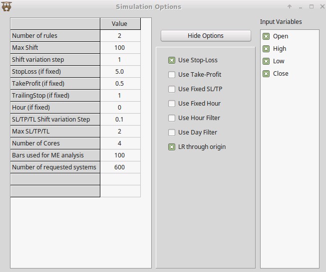
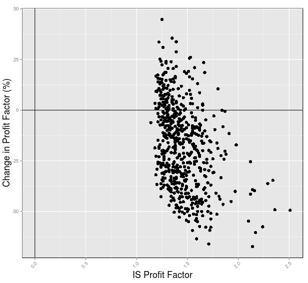
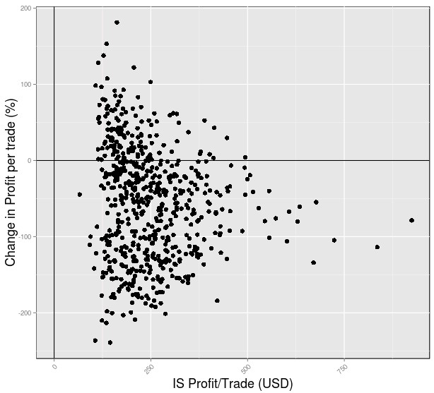
For this exercise I used EURUSD 1D to mine 600 trading systems under the conditions showed in the options dialog above. I performed the mining process from 1986 to 2001 and kept the final 15 years of data in order to perform the pseudo out-of-sample analysis. After the mining process is finished you can right click on the results grid and save a CSV file with all the results. The csv file will include the in-sample statistics plus all the pseudo out-of-sample statistics which are not showed in the regular results grid. The R code showed in the first part of this post allows you to plot the deterioration of these statistics relative to their in-sample values. In this case I included plots for the deterioration of the profit per trade and the profit factor since these are some generally interesting characteristics to look at.
As you can see in the two plots below in this case the deterioration of the profit per trade and the profit factor across 15 years of pseudo out of sample was quite significant, which is normal. As you can see the largest profit factors and profits per trade under in-sample condition tend to deteriorate the most while more intermediate values tend to deteriorate in a rather random manner with a small percentage of systems even showing an improvement over the in-sample conditions. Of course some systems will show improvements because they will – by pure chance – be more adapted to the conditions that followed than the market conditions used to create them.
–


–
The average deterioration values were -56.86% for the Profit per trade and -17.41% for the profit factor. This means that if you traded a portfolio of all the 600 systems in an equally weighted manner your profit per trade after 15 years would deteriorate by a bit more than half while your profit factor would deteriorate by about one fifth. This means that you would still have an expectation to be profitable but you would take losses on many systems that would deteriorate very substantially. For example systems that have net negative results see deterioration of their Profit per trade in the -100% and further region. As I have mentioned before you can use this type of measurement to make very general observations but do not try to narrow down a mining criterion that generates only systems that do not deteriorate because you will be fitting to randomness, introducing mining bias in the pseudo out of sample analysis. If you would like to learn more about system mining and how you too can learn to analyse and build your own trading portfolios please consider joining Asirikuy.com, a website filled with educational videos, trading systems, development and a sound, honest and transparent approach towards automated trading.


