Mechanical Forex

Evaluating the on-going performance of a trading strategy is a complicated task since expectations about a system’s performance are often defined by spans of time that are much larger than those considered in live trading. In order to successfully draw correct expectations based on the amount of time that has being traded it becomes fundamental to correct measures so that they reflect what is expected from any given live trading period. On today’s post we are going to learn how to perform this type of corrections using python and the qq-pat library in order to draw better expectations and worst cases for any given live trading period using information from long term back-testing results. We are going to go through an example using the Sharpe ratio but you can definitely use  any other statistic you want in order to draw the same conclusions. You can download this file to reproduce the results from this post.

–

#!/usr/bin/env python
#Created by Daniel Fernandez
#http://mechanicalforex.com 2015

import numpy as np
import pandas as pd
import csv
import datetime
import qqpat
from random import randint
import matplotlib.mlab as mlab
import matplotlib.pyplot as plt

NUM_SAMPLES = 400
WINDOW_SIZE = 100
BINS_TO_USE = 20

def lastValue(x):
    try:
        reply = x[-1]
    except:
        reply = None
    return reply

def main():

    tradeTimes = []
    tradeBalance = []

    with open("results.txt", 'rb') as csvfile:
         reader = csv.reader(csvfile)
         i = 0
         for row in reader:
             if i > 0:
                 tradeTimes.append(datetime.datetime.strptime(row[3], '%d/%m/%Y %H:%M'))
                 tradeBalance.append(float(row[10]))
             i += 1         
           
    returns = pd.Series(data=tradeBalance, index=tradeTimes).resample('D', how=lastValue).pct_change(fill_method='pad').fillna(0)
    analyzer = qqpat.Analizer(returns, column_type='return')
    overall_sharpe = analyzer.get_sharpe_ratio()[0]
    analyzer.plot_analysis_returns()
    
    print "Sharpe for entire backtest is {}".format(overall_sharpe)
    sharpes = []
    
    for i in range(0, NUM_SAMPLES):
        selected_index = randint(0, len(returns.index)-WINDOW_SIZE)
        data = returns[returns.index > returns.index[selected_index]]
        data = data[data.index < returns.index[selected_index+WINDOW_SIZE]]
        analyzer = qqpat.Analizer(data, column_type='return')

        sharpe = analyzer.get_sharpe_ratio()[0]
        
        if sharpe != float("NaN"):
            sharpes.append(sharpe)    

    #very roughly approximate worst case
    print "Worst case at 99% confidence is {}".format(np.asarray(sharpes).mean()-4*np.asarray(sharpes).std())     
      
    # the histogram of the data
    n, bins, patches = plt.hist(sharpes, BINS_TO_USE, normed=1, facecolor='green', alpha=0.75)

    # add a 'best fit' line
    y = mlab.normpdf( bins, np.asarray(sharpes).mean(), np.asarray(sharpes).std())
    l = plt.plot(bins, y, 'r--', linewidth=1)

    plt.xlabel('Sharpe ratio')
    plt.ylabel('Probability')
    plt.title('Sharpe ratio histogram')
    plt.grid(True)
    plt.show()
             
if __name__ == "__main__": main()

–

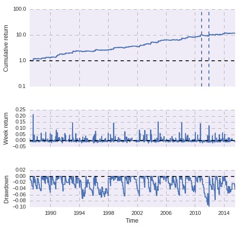
You have finished the simulations of your system across 30 years of data and you’re now happy with what you have. Your system has a nice equity curve and an overall Sharpe ratio of 0.68. You start trading your strategy and after 100 days your sharpe ratio is -2, surely something must have gone wrong in the process! How can a system that had a 0.68 Sharpe ratio in simulations of over 30 years show a Sharpe ratio of -2 after 100 days? You must have definitely made some kind of mistake within your testing process. Or did you?

The main issue with the above case is that you’re comparing a statistic that took 30 years to generate with a statistic that you have derived over merely 100 days of data. This means that you’re assuming that the value of the statistic will converge to its long term equivalent in 100 days, something that is basically incorrect the vast majority of the time, especially when dealing with trading systems where the distribution of returns is quite simply not homogeneous. In this case what we must do to derive a correct expectation is to see how cases for a given statistic are distributed within our long term statistics. We can easily do this using python and the qq-pat library.

–

–

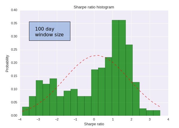
If you wanted to know what Sharpe ratio values you should expect within a 100 day period for any trading system you should perform a random sampling of 100 day periods from your long term back-testing data in order to see which values are to be expected. After getting the data into a pandas array we can go through a loop and take 400 samples (although you can take more, the more the better) from the backtesting data and then calculate the Sharpe ratio for each one of these periods. After we have derived all the different Sharpe ratios we can then build a distribution that shows us what Sharpe values we can expect from this process.

Certainly the distribution of Sharpe ratios reveals that the 30 year case is really a relatively rare occurrence within a 100 day period. We are much more likely to see a Sharpe ratio above 1 than to see a value of 0.68 and we also have a very significant probability to see a Sharpe ratio below zero. A Sharpe ratio of -2 – what we saw in our hypothetical case – is well within what is expected for this system within a 100 day period. Therefore it would be very wrong to say that the Sharpe ratio has “deteriorated” if you obtained a Sharpe ratio of -2 within 100 days of trading for this strategy because this is simply within the realm of possibilities for this strategy. With this curve it is evident that you can expect values up to -4 for the trading system, but even then a value of -5 may not be low enough to mean that the Sharpe ratio has deteriorated significantly. You can draw a very approximate worst case using the 4 sigma level of the distribution, which would give you a worst case Sharpe ratio of  -6.8 for the 100 day period.

–

–

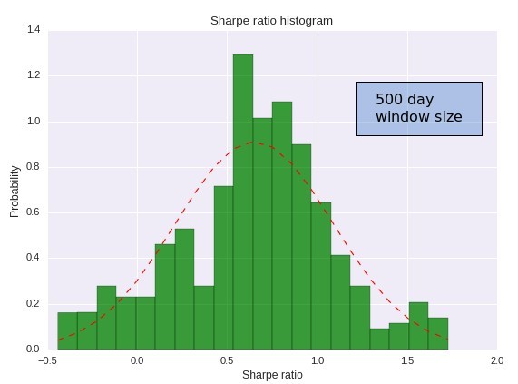
If we change our window size you can also see how the Sharpe ratio starts to converge more heavily towards the 30 year value. Here the largest probability starts to fall towards the 0.6 region but we still have a very significant probability to achieve a much worse Sharpe. In this case – when the distribution behaves much more like a normal distribution – we can use the 4 sigma worst case in a more justified manner and we can say that the 99% confidence level for discarding the strategy is at a sharpe level of -1.10. As you can see within a 500 day period we have a much lower tolerance for having bad results when compared with a 100 day period.

The above shows us that the long term statistics of our strategy are not a good source of judgement when determining whether our strategy is or is not working according to it’s past behavior. Since market conditions have varied so much within long term back-testing periods it becomes imperative to do some sort of sampling from the data in order to derive distributions of the statistic that interests us so that we can draw realistic expectations of what the strategy has to offer at different time spans. Comparing very long term statistics with short periods is simply wrong because a long term back-testing period contains many possible values for a given statistic across a shorter time span.

If you would like to learn more about evaluating systems and how you too can draw worst cases for evaluating and discarding trading strategies  please consider joining Asirikuy.com, a website filled with educational videos, trading systems, development and a sound, honest and transparent approach towards automated trading.