The portfolio optimization problem has been one of the most studied problems in risk management during the past century. From the research published by Markowitz in the 1950s there have been significant improvements in the way in which we do mean-variance optimizations and the algorithms used to solve the quadratic optimization problem. Today I want to share with you some code for the finding of the minimum variance portfolio in python as well as some comparisons between the different algorithms that we have available for the calculation of such portfolios. For this I will be using the CVXPY library which is undoubtedly the best library for solving this type of problem in python. We will go a bit through the code and the results of the different algorithms available through the CVXPY implementation.
–
from cvxpy import *
import pandas as pd

def calculate_portfolio(returns, selected_solver):

    cov_mat = returns.cov()
    Sigma = np.asarray(cov_mat.values)
    w = Variable(len(cov_mat))
    risk = quad_form(w, Sigma)
    prob = Problem(Minimize(risk), [sum_entries(w) == 1, w > 0])
    prob.solve(solver=selected_solver)

    weights = []
    for weight in w.value:
        weights.append(float(weight[0]))

    return weights
–
Optimizing a portfolio is quite straightforward: simply find the weights that you need to give to each one of the systems such that some underlying portfolio property is either minimized or maximized. Some of these procedures cannot be easily solved analytically and therefore require some form of iteration – such as when you’re looking for the best historical Sharpe – but other types of optimizations such as the minimum variance portfolio can indeed be solved analytically using the covariance matrix. The code above shows you how you can obtain the minimum variance portfolio given a pandas DataFrame containing all the system returns and a selected_solver coming from the list that you can obtain from the installed_solvers() command (for example CVXOPT).
As you can see the great advantage of the CVXPY library is that the problem is expressed in a way that is closer to what you would write on a piece of paper if you were explaining the math, rather than in the matrix form that is usually required by the direct use of the optimization libraries. The CVXPY project does not directly implement any optimization libraries but it simply serves as a great wrapper to enable the use of all these underlying libraries with the same input format and with a more intuitive set of instructions. For example in this case I simply tell it that I want to minimize Risk and I want the sum of weights to be 1 and all of them to be greater than 0.
–

–
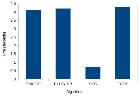
Given that we can very easily switch between optimizers it becomes very easy to perform benchmarks of the optimization using the different available solvers. The above image shows you the amount of time it takes in seconds to solve the minimum variance problem using the 30 year monthly returns of 500 trading strategies with the 4 different solvers that are available after you install CVXPY. As you can see the SCS solver is by far the best one – not surprisingly since it’s coded in C – with a performance that is almost 10x that of the more commonly used CVXOPT algorithm. Accuracy in SCS is also not worse with the Sharpes and weights achieved by the SCS algorithm being basically equal – mostly even better – than those achieved by the other algorithm types. The differences between CVXOPT, ECOS and other native python libraries is basically small as it’s not possible to remove most of the overhead unless most of the code is executed using a non-interpreted language like C.
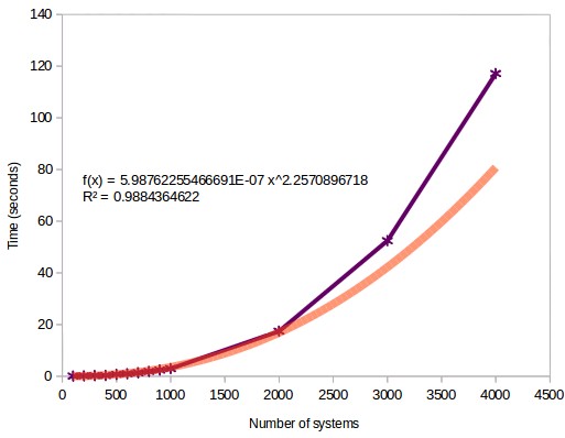
With the knowledge that the SCS algorithm is the best one we can now evaluate the computational cost of performing portfolio optimizations using different system numbers. As you can see in the image below the computational cost increases as a power law function as the number of systems increases. However as you can see the fit is very good in the beginning but the estimation starts to become worse as the number of systems goes beyond the 2500 system mark. This is possibly because the arrays become big enough for data transfers and the calculation of the covariance matrix to start to add significantly to the overall program execution cost. As the number of systems starts to be come much greater than the number of returns we start to get some important problems with the calculation of the covariance matrix. In the case of 4000 systems using 30 years of monthly returns we have 360 return values but 4000 system values, we start to see these instabilities in the covariance matrix.
–

–
Another problem we have discussed before is that the sample covariance matrix – the one we derive from the historical returns – is bound to have a lot of estimation error and therefore a lower performance in the out-of-sample when compared with naively optimized portfolios (for example equally weight portfolios), especially when there are a high number of uncorrelated strategies. There are some ways we can try to work around this that also help us reduce the problems we get when the number of strategies is greatly superior to the number of sample returns. Some of which we will be exploring within future posts. If you would like to learn more about portfolio optimization and how you too can trade very large system portfolios please consider joining Asirikuy.com, a website filled with educational videos, trading systems, development and a sound, honest and transparent approach towards automated trading.strategies


