Mechanical Forex

During the past two years I have been an avid fan of the quantopian platform. Not only do they allow you to back-test your stock strategies with 1M data quality but they also allow you to live trade your strategies on Interactive Brokers or Robin live trading accounts. However one thing that has always bugged me is how there is simply no feature to export the back-testing results from the platform and you’re simply stuck with the graphs and analysis from their back-testing page which are rather limited and difficult to adapt to presentation needs — at least from my perspective. On today’s post I am going to share with you a trick that allows you to export your daily return back-testing results from quantopian and I will also show you how you can then analyze the results in a more flexible environment, like a script running qqpat.

–

bt = get_backtest('57707ded4a4d9gh0f8df4b5ea')
returns = bt.daily_performance.returns
for i in range(0, len(returns.index)):
    print "{}, {}".format(returns.index[i].strftime("%Y-%m-%d"),returns.ix[i])

import pandas as pd
import datetime
import csv
import qqpat

def lastValue(x):
    try:
        reply = x[-1]
    except:
        reply = None
    return reply
    
tradeTimes = []
tradeReturn = []

with open("/pathtofile/filename.csv", 'rb') as csvfile:
    reader = csv.reader(csvfile)
    for idx_data, row in enumerate(reader):
        if idx_data > 0:
            tradeTimes.append(datetime.datetime.strptime(row[0], '%Y-%m-%d'))
            tradeReturn.append(float(row[1]))      
    data = pd.Series(data=tradeReturn, index=tradeTimes)
            
data = data.fillna(0.0)
                                     
analyzer = qqpat.Analizer(data, column_type='return', titles=["system"])

analyzer.plot_analysis_returns()
analyzer.plot_analysis_rolling()
analyzer.plot_monthly_returns_heatmap()
analyzer.plot_annual_returns()

–

Analyzing back-testing results in a custom environment is fundamental to trading success. While the quantopian platform provides some fundamental data such as the comparison against the SPY, the Sharpe, the beta and alpha coefficients, it fails to give some other fundamental information such as the R², the yearly returns, the monthly return heatmaps, etc. Of course a single program will struggle to give any user everything he or she wants for statistical analysis and this is the reason why being able to export results is so important. Even when using their notebook, analysis is limited by the libraries they allow you to import and sadly a useful library such as qqpat is still not available (they do offer pyfolio but again it is hard to give everybody, everything they want).

To be able to export data from quantopian I used a simple trick using their notebook — showed above. Since they allow you to import daily return results from backtests I then used a simple loop to print all the values from the returns in a manner that generates a text block with all the information we need. You can then take that generated text block and copy-past it into a blank file and save it as a csv. The generated file contains a column with the date values and another with the returns matching that date.  It is worth mentioning that I couldn’t find anything in the quantopian TOS against using this type of procedure. It would be surprising if there was given that the generated return data from your own trading systems is hardly worth protecting from you — who created the system.

–

–

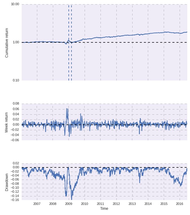
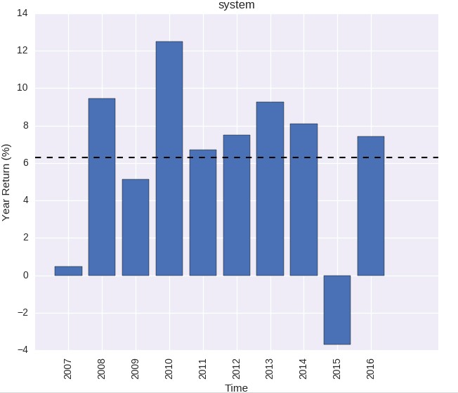
Once you generate the file you can then proceed to analyze the results using qqpat. The above python script loads the data from the csv (change the path to the path of your file) and creates some important plots. The above PerformanceAnalytics style plot is generated by using the plot_analysis_returns function while the following functions generate the 12 month rolling performance analysis, the monthly return heatmap and the annual return plot (showed below). I find annual return plots and monthly heatmaps especially useful since they allow you to grasp how homogeneous a strategy is in time. The underwater plot in the returns plot is also very useful since it allows you to easily see where the worst drawdowns have been located historically.

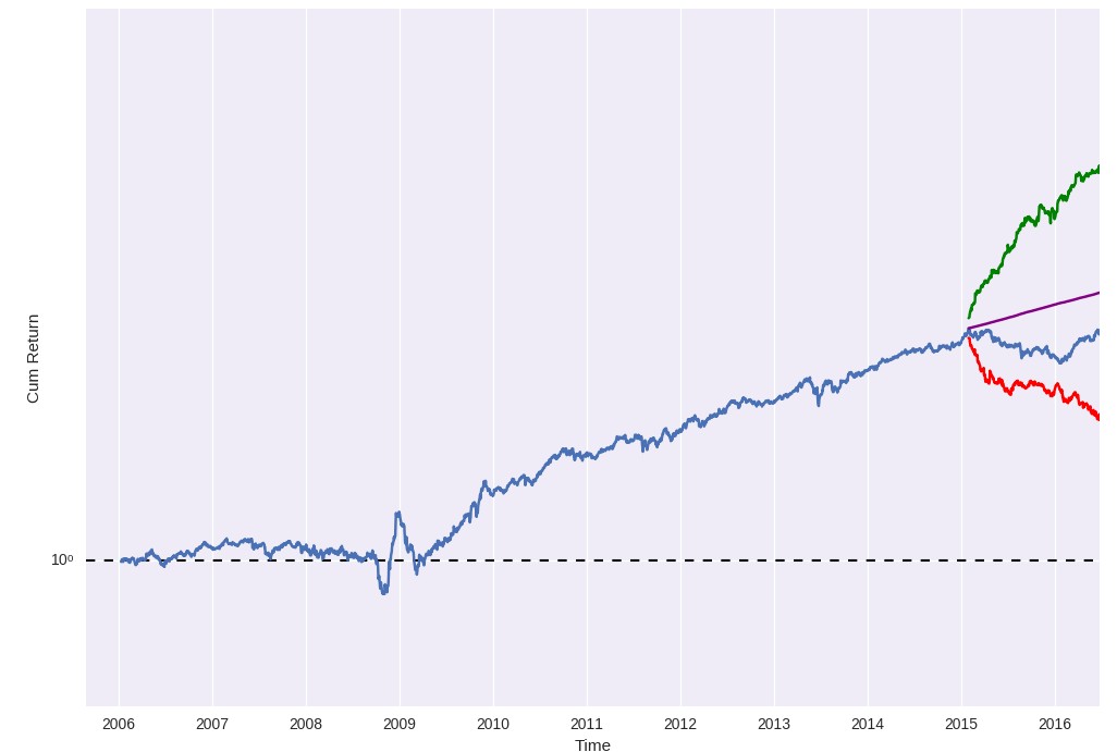
Of course you’re not limited to just using these functions within the script but you can use any of the functions available in qq-pat. For example you can easily use get_mc_statistics_for_current_dd to see if the current drawdown period falls within a Monte Carlo worst case scenario calculated at the specified confidence interval.You can also use the plot_mc_limits function to obtain a plot of the worst and best case values at each point in time for the last drawdown at the specified confidence (this plot is also showed below). With this plot you can take a look at the red line and instantly see if your strategy has ever gone beyond a worst case scenario balance within its last drawdown period.

–

–

Most importantly now that the data is within a csv file you are only limited by your imagination in how you can analyze it. You can use qq-pat for some powerful analysis but you could also get your results into R and analyze them using a library such as quantmod or PerformanceAnalytics or you could code your own functions with any libraries you want to import in python to come up with your own idea of what the perfect analysis looks like. In any case, having the data allows for a flexibility that simply is not possible if you’re limited to using python notebooks within the quantopian platform. If you would like to learn more about my work and how you too can learn how to design, analyze and trade strategies please consider joining Asirikuy.com, a website filled with educational videos, trading systems, development and a sound, honest and transparent approach towards automated trading.strategies.