Given the fact that predicting future system performance from in-sample system statistics is extremely difficult it is interesting to look at other potential relationships that may allow us to forecast system performance. Since trading system results depend fundamentally on how the market behaves it is therefore interesting to consider whether a relationship between previous market conditions and future performance can be established. Today we are going to take a look at the relationship between the fractal dimension and the returns of a trading system and try to establish whether this specific trading system is more prone to take losses under some types of market conditions. This might yield some interesting results, such as the possibility to use a fractal dimension based filter to avoid losing periods. Of course I am using this trading system as a simple sample case, other systems might show different results. If you are an Asirikuy member you can use any NST back-test and NST 1H data files to reproduce the analysis below.
–
# Sample script to calculate
# fractal dimension values for a set of system returns
# Daniel Fernandez
# http://mechanicalforex.com
# https://asirikuy.com
# 2016

library(pracma)
library(quantmod)
library(fractaldim)
library(ggplot2)
library(e1071)
library(reshape)
library(PerformanceAnalytics)

calculate_fdim <- function(fxdata, number){

  method <- "rodogram"
  colnames(fxdata) <- c("data")
  fractal_dimension_for_symbol <-fd.estimate(as.data.frame(fxdata$data)$data, method=method, trim=TRUE, window.size=number)$fd
  data <- c()

  return(fractal_dimension_for_symbol)
}

path <- paste("/pathToData/EURUSD1987_60.csv", sep="")
fxdatatemp <- read.zoo(path, sep = ",",format="%d/%m/%y %H:%M", header=FALSE,index.column=1)
fxdata<- as.xts(fxdatatemp)
colnames(fxdata) <- c("open", "high", "low", "close", "vol")
fxdata <-fxdata$close

resultsTEMP <- read.zoo("/pathToTest/sys1.txt", sep = ",",format="%d/%m/%Y %H:%M", header=TRUE,index.column=1,colClasses=c("NULL", "NULL", "NULL", "character", "NULL", "NULL", "NULL", "NULL", "NULL", "NULL", "numeric", "NULL", "NULL", "NULL"))
results<- as.xts(resultsTEMP)
daily <-dailyReturn(results)
daily <- na.fill(daily, fill = 0.00)

for (i in 1 : length(daily)){
  fxdata_used <- fxdata[index(fxdata) < index(daily)[i]]
  fxdata_used <- tail(fxdata_used,2000)
  daily$fractal[i] <- fd.estimate(as.data.frame(fxdata_used$close)$close, method="rodogram", trim=TRUE)$fd
  print(daily$fractal[i])
}

hist(daily$fractal, xlab="Fractal dimension")

p <-ggplot()
p <- p + geom_point(size=1.5, aes(x=as.numeric(daily$daily.returns*100) ,y=as.numeric(daily$fractal)))
p <- p + ylab("Fractal dimension")
p <- p + xlab("Return (%)")
p <- p + theme(axis.title.y = element_text(size = rel(1.5)))
p <- p + theme(axis.title.x = element_text(size = rel(1.5)))
p <- p + theme(axis.text.x = element_text(angle = 45, hjust = 1))
p <- p + theme(panel.background = element_rect(colour = "black"))
p <- p + geom_abline(intercept = 0, slope = 0)
p

comp <- merge(daily$daily.returns, daily[daily$fractal < 1.50 | daily$fractal > 1.51]$daily.returns)
comp <- na.fill(comp, fill = 0.00)
charts.PerformanceSummary(comp, ylog=TRUE)
–
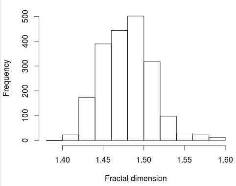
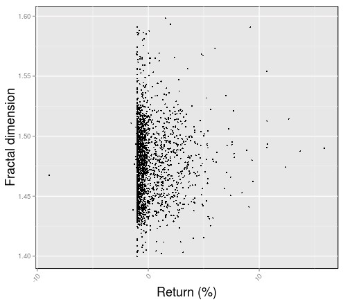
If the ability of trading systems to predict future market conditions depends on whether the market behaves randomly or not then there might be some relationship between properties that change as a function of market predictability and trading system returns. The fractal dimension – which we have discussed extensively on this blog – changes as a function of the relationship between the elements of a time series and is therefore adequate as an initial test to address this hypothesis. To do this I have used the R script above where the fractal dimension of the 1H timeframe for the past 2000 bars is calculated for each daily return value for a loaded trading strategy returns. In the end an xts series is obtained with both the system returns and the fractal dimension value calculated for the past 1H bars preceding that return value.
The graphs below show the distribution of the fractal dimension values and the scattering plot of system returns Vs fractal dimension. As you can see most fractal dimension values are located close to the 1.5 area, reason why the scatter plot shows most returns around this zone on the scatter plot. Since the system uses a stop-loss you can see how most negative returns are cut-off close to the 1% loss level except for cases where price slipped – due to price gaps – with a sole return at around -7% present due to this reason. There is no evident linear correlation between the fractal dimension and system returns with a correlation coefficient of 0.02 between both values.
–


–
There are some regions where there are some larger concentrations of positive Vs negative returns (for example between 1.5 and 1.51) and removing those type of regions can bring a slight improvement to trading results, as showed in the image below. However this improvement in trading cannot be said to be statistically significant as it is just a cherry picked result region from the fractal dimension analysis. Moreover this region is not coherent across many different EUR/USD systems, meaning that it does not even constitute a set of market conditions where a large portion of systems are expected to show poorer results. For each particular system there is always some region that shows a larger number of negative Vs profitable returns but this would be expected simply due to random chance and making trading decisions based on this data would be naive.
That said there are many things that can be varied in this analysis that may change the outcome it presents. I have arbitrarily used a 2000 window to calculate the fractal dimension but shorter or larger windows may show substantially different results, as it has happened in the past with similar types of analysis. The market condition characteristics a system might be sensitive to might match its trade horizon window or some other system characteristic. I have also used the rodogram algorithm for the calculation of the fractal dimension but this algorithm can be changed and the results may also change substantially due to this reason.
–

–
Of course the above is just the start. Other variables such as the Hurst exponent and approximate entropy can also be used in a similar way. There is a lot of research that can be done in this area including the exploration of commonalities between different systems and their return/market condition relationships – as expressed by the above mentioned variables – as well as the construction of machine learning models to relate returns and market conditions. If the relationships between market conditions are returns are complex – as we might expect them to be – then we might need to use more powerful models to describe them. If you would like to learn more about trading systems and how you too can create and analyse your own strategies please consider joining Asirikuy.com, a website filled with educational videos, trading systems, development and a sound, honest and transparent approach towards automated trading.strategies


