Reinforcement learning (RL) has been an important focus for me since I finished my machine learning nanodegree at Udacity. This is because reinforcement learning is substantially different from our other machine learning strategies – which use moving window supervised learning approaches – and therefore a potentially important source of diversification for our trading. However it is often very difficult to understand how reinforcement learning systems work and perhaps more importantly, to be able to predict what sorts of actions they might take given some market conditions. Today I want to offer you a peak into the brain of a Q-table reinforcement learning algorithm so that we can take a look into what it ends up doing and how it ends up making trading decisions.
–

–
When I started studying RL approaches in trading it soon became clear that you cannot just throw powerful RL approaches at the market and expect useful algorithms. An RL algorithm can very easily curve-fit to noise and can generate results that are not general and basically the result of data-mining bias (you can read more about that here). For this reason the successful algorithms we have found have turned out to be Q-learning approaches that are simple enough as to be represented and understood in a graphical manner.
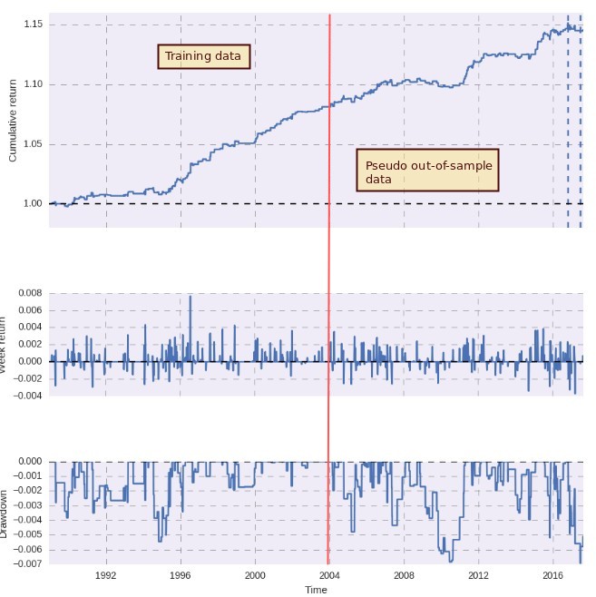
To put it simply our algorithms study a set of pre-established market conditions – market states – that are defined by the state of a set of predefined variables. In a very simple case if you had just one variable, say yesterday’s price, you could define three market states, yesterday was bullish, yesterday was bearish or yesterday was neutral. This would create a q-table with three entries and the algorithm will train through the market data assigning rewards depending on the profits/losses generated by going long, short or staying out of the market. Generally we use 60% of our data to train the algorithm – where it’s executed 10 times to refine the Q-table – and we then execute it one time across the entire data. This means that improvements in the pseudo out-of-sample period can only be made with training without hindsight (the algorithm just learns from what it’s doing not from the future in any way). The first image in this post shows the balance curve resulting from carrying out this process with one of our RL algorithms.
–

–
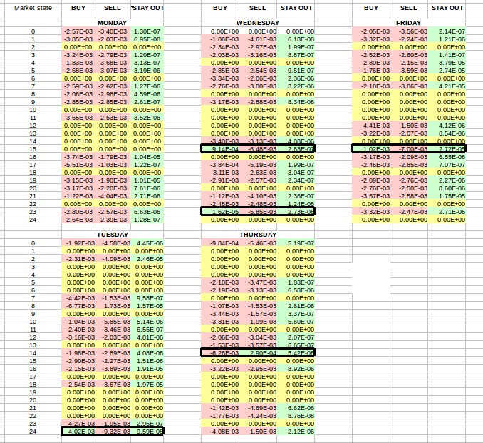
Since this Q-learning approach generates a Q-table we can explore what the algorithm learned by looking at the values of this table and color coding them according to their sign. The image above shows you the result of doing this. In the case of this algorithm we have 25 different market states that are each separated as well by the day of the week. This means that in total we have 125 possible market states. As you can see in most cases the algorithm is deciding not to trade as it has learned that – per its market state definitions – trading most of the time does not reliably lead to profits. This is why most BUY/SELL rows are negative – the algorithm expects a negative reward from trading under these conditions – while the STAY OUT row is always green. Some rows are yellow because these market states never presented themselves across the entire testing process.
However there are clearly some exceptions, otherwise the algorithm would never trade. The exceptions are highlighted in black border boxes so that you can see them more easily. We have mainly five instances where the algorithm has decided that trading is better than staying out of the market, four that trigger long positions and another that triggers a short position. For state 15 we can see that this generates a long signal on both Friday and Wednesday while for Thursday and Tuesday the algorithm determined that the edge it received is not large enough. With this info we can see that the algorithm will never trade on Mondays and will take only long trades on Tuesday, Wednesday and Friday and only shorts on Thursday. We can also see that the q-table value is highest for Friday state 15, implying that this behavior will be the hardest to change (and should be the most profitable if what has been learned is not curve-fitted). Wednesday is also the only day with two states that can generate positions.
–

–
Although the behavior of reinforcement learning algorithms can be a bit puzzling we can perform some basic and graphical analysis on simple Q-learning algorithms to learn more about how they trade and what the result of the trading process is. With this we can get some expectations about how the algorithms trade and how well ingrained the trading behavior actually is (by comparing the magnitude of the values), something that can be harder to do with other types of machine learning algorithms. The above shows that complexity is also unnecessary to get profitable historical results. Well chosen market state descriptors can lead to successful strategies with much less risk of over-fitting or high data-mining bias.
If you would like to learn more about reinforcement learning and how you too can create strategies that constantly learn from new market conditions please consider joining Asirikuy.com, a website filled with educational videos, trading systems, development and a sound, honest and transparent approach towards automated trading.strategies.


