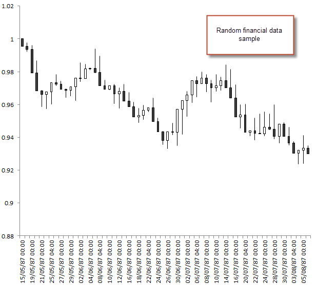
On my last post I described how to use the R statistical software in order to generate simple random financial data series. Today we are going to use these series in order to test the data-mining bias of an automatic system generation approach in order to determine what system characteristics are required to assert that a strategy is most likely not the result of spurious correlations. Although I have approached the data mining bias problem on some Currency Trader Magazine articles (particularly using random variables to test for only spurious correlations), this approach – using random synthetic data – offers us a complete dimension regarding the interaction of the OHLC variables within the system creation process, something that the other approach neglects. Within the next few paragraphs and posts I am going to share with you my experience with this testing procedure based on random data, as well as my conclusions regarding its use in Kantu (my system generator program). You can get the random data used for these articles here and you can also download the Kantu demo to test this approach yourself.
–
–
So what is a data-mining bias? When you create strategies in an automatic fashion you face the problem of not being able to know the probability that the generated strategy is the mere result of a spurious correlation that is achieved simply because your mining process is able to get anything outside of the data. As the saying goes, buy a heart lyrics “if you torture the data long enough, it will confess to anything”, meaning that if you perform data mining with enough degrees of freedom for a long enough time you’ll always be able to find a system that has whichever level of profitability you desire, up to the maximum profit that can be extracted from the market historically. Think about this, if you have a strategy that can have “and/or” conditions, it can easily be demonstrated that there is always a set of rules that can be profitable on every candle and extract all possible profit within some historical data. Given infinite degrees of freedom, there is always a fit for every problem. Therefore, for a data-mining approach with infinite degrees of freedom the data-mining bias is the greatest, you’ll always be able to find a strategy on a random time series with the same profitability as the strategy you have developed on your real historical financial data.
However, as soon as you restrict the degrees of freedom on a data mining approach you reduce the data-mining bias to a smaller level. If your data mining process only generates systems with two rules it will be impossible for it to extract all possible profits from the market and the amount of profit it will be able to extract from random data series will be limited significantly. The idea of using random time series is to be able to answer a simple question: What are the best statistical characteristics that my system can achieve if it can only generate spurious correlations? Once you have the answer to this question – which is your data-mining bias – you will be able to evaluate whether the strategies you generate using real financial time series are bound to be significant. Your data-mining bias depends on the degrees of freedom of your data-mining process (how many rules, how many possible shifts, which exit mechanisms, how many parameters, etc) and it also depends on the amount of data being used. For this reason you need to repeat your analysis for any changes across these aspects.
Data length is a very important part of the question. Whenever you have more data the data-mining bias is reduced because the probability to find a spurious correlation that is present across the whole data set is diminished. A system that would have a significant chance of being chosen out of luck within a 5 year period may be extremely difficult to find out of luck within a 10 year period, a system that would be chosen out of luck on one symbol’s 10 year data may be incredibly hard to find within 4 symbols on the same data length (because in practice the system would need to work under 40 years of random data). For this same reason the TF is also important, the lower the TF, the lower your data mining bias (other problems – like broker dependency – start to be present as well so that must be taken into consideration).
–
–
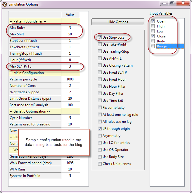
To test for our data mining bias in Kantu we need to first select the conditions we want for the creation of trading strategies. Using different inputs or using different rules and shift limits changes the magnitude of our testing bias. We must also make sure that the random data we generated matches the length we want to test on our real data series and we need to ensure that the same entry/exit mechanisms are present. In the examples I am going to use I have generated random data for 25 years of daily data and will be generating strategies using a maximum shift of 50, a maximum set of 3 price action based rules and a stop-loss for the exits of the trading strategy. We will also restrict the rules to use only the Open/Close values for the strategy. You can also run experiments using different system generation options, to see how the degrees of freedom you give your strategy changes your data-mining bias.
buy priligy south africa It is also important that you record the amount of attempts used to generate the strategies, because the confidence in your data-mining bias measurement depends on how exhaustive your search of the logic space is. If you just run 1000 random system simulations and you find that the best possible system has certain characteristics, you’ll have much less confidence than if you generate 10 million strategies. The amount of systems you need to generate to have good confidence depends on your degrees of freedom and grows exponentially as the possibility of more complex systems becomes larger. If your logic space is in the order of 1000 trillion it will be extremely hard to come to any realistic conclusions regarding the data-mining bias. For the logic space I chose for these experiments (SL = 0.5-3.0 in 0.5 steps, OC 3 rules, max shift 50), there are about 167 million possible strategies (shift step 4, see comments for a breakdown of this calculation) so we should generate at least this number of systems in our random-data test to have some confidence in our data-mining bias. A good strategy to reduce the logic space complexity is to increase the steps of variables (for example round shifts to the nearest 5), to reduce the number of inputs or to allow for a smaller range in the SL/TP/TL searches.
Another important aspect is to use more than one random data series for the tests. Doing several tests on different random data sets can increase your confidence regarding the possibility to generate certain results. A single random data set might have some quirks (especially if the data is not very long) so it is desirable to repeat the analysis on several different sets. Now that we have a predefined setup we can run our tests and see what we obtain, we can then compare these results to the system generation results of Kantu on a real financial data symbol and see whether we can obtain systems above our data mining bias. Tomorrow we’ll go into the second part of this series where we’ll see some real results for this analysis. Any suggestions? Leave comment!
If you would like to learn more about algorithmic system generation and how you too can use Kantu to generate strategies for your trading please consider joining Asirikuy.com, a website filled with educational videos, trading systems, development and a sound, honest and transparent approach towards automated trading in general . I hope you enjoyed this article ! :o)


Marcos’ suggested technique is to split the totality of the data set into N equal-length chunks, each big enough to cover all the serial covariances and suspected mean-reverting behavior. Then build all the permutations of the chunks. For each permutation, run your exhaustive systems’ optimizations on the first half of each permutation’s chunks (the in-sample), and record the system’s results on the other halves (out-of-sample). If the in-sample-best optimized systems’ performances out-of-sample are less than the median out-of-sample performance of the systems, then the optimization process and/or system itself is overfit.
Hi Experquisite,
Thanks for your comment :o) This is in essence a walk forward technique (use N chunks and perform in/out of sample analysis on each one, then see if the process worked across the board). I can imagine that this works for system optimization but it doesn’t work for a system building approach because I can eventually come up with a technique that generates good OS results across all chunks, because I have massive system building abilities and whatever number of degrees of freedom I desire. In essence since I have so much fitting power I can indeed perform this experiment as many times as necessary with different building paradigms and get whatever result I desire.
I believe that this type of techniques designed for system optimization are not suited for system generation using data-mining with modern computer capacity. I am now much more convinced that Bob’s suggested approach might be best. Generate a data-mining bias and simply see if you can come up with something that is better. Thanks again for commenting :o)
Best Regards,
Daniel
Daniel
I’m not sure how exactly you’ll do this. I could think of two ways somehow complying with your text. Can you provide a simple/generic step by step?
Best,
Nuno
Hi Nuno,
Thanks for commenting :o) Let me know which specific things you would want me to explain better and I’ll clarify,
Best Regards,
Daniel
[…] how much should you reduce complexity? The data-mining bias exercise we did before using kantu (see here and here) gives a relatively small data-mining bias of 0.2-0.4 Profit/MaxDrawdown over a 25 year […]
How did you get 121 million possible strategies using SL = 0.5-3.0 in 0.5 steps, OC 3 rules, max shift 50? With a shift step of 5, the total number possible strategies I computed was 45366300. The number was 227799000 if the shift step is 4. I believe I used the same formula that gave me the correct number in the example count in the manual of OpenKantu.
Thanks for clarifying.
Hi Tommy,
Thanks for writing. This 121 million value was for a shift step of 4, but the result is actually 167 million (I have now corrected the mistake within the post). Here is the calculation broken down:
number of SL possibilities = 6
number of possible inputs = 2 (Open and Close)
number of available shifts = 12 (1 to 50 in 4 step [1, 5, 9… 49])
number of shift permutations with repetition = 144
number of input permutation with repetition = 4 (O > C, O > O, C > O, C > C)
number of potential rules per rule = 576
number of invalid rules (see below) = 24
number of valid rule combinations without repetition for 3 rules = 27,880,600
total number of potential scenarios = 167,283,600
In your calculation you should consider that rules should always be of the form input1[shift1] > input2[shift2], you should also consider that rules where the input AND the shift are equal are invalid (for example open[50] > open[50]) and you should also consider that when calculating the potential number of rule combinations the rule order does not matter (rule1, rule2, rule3, is the same as rule2, rule3, rule1) and rules should not be repeated. I hope this answers your question. Thanks again for writing,
Best Regards,
Daniel
Hi Daniel,
Thanks for the explanation. I agree with the method of your calculation. We should arrive at the same answer but I think each of us made a mistake:
1. I thought the number of SL possibilities was 5 but actually it should be 6.
2. There were actually 13 possible shifts (1, 5, 9, …, 41, 45, 49).
So the number of valid rules for a single rule is 650. The number of combination for 3 rules is 650 choose 3 = 45559800. With 6 different SL levels, the total number of rules using this calculation should be 273358800.
I think this should be correct now.
Best,
Tommy