Lake Magdalene Let’s start the week with some good news :o). During the past 2 years the development of machine learning systems has been a big priority for me. These techniques offer us the dream of permanently self-adapting trading implementations where trading decisions are constantly adjusted to match the latest data. Although I am aware that even this level of adaptability does not guarantee any profitability – as the underlying models may become useless under some new conditions – it does provide us with a larger degree of confidence regarding our ability to predict a certain market instrument going forward. On today’s post I am going to show you my latest development in the world of neural networks, where I have finally achieved what I consider outstanding historical testing results based on machine learning techniques. Through this article I am going to discuss the different methods that went into this new system and how the key to its success came from putting together some previously successful – yet not outstanding – trading implementations.
–
–
First of all I would like to describe the way in which I develop neural network strategies so that you can better understand my systems and latest developments. My neural network trading systems are designed so that they always retrain from newly randomized weights on every new daily bar using the past N bars (usually data for about 200-500 days is used) and then make a trading decision only for the next daily bar. The retraining process is done on every bar in order to avoid any curve fitting to a given starting time or training frequency and the weights are completely reset to avoid any dependence on previous training behavior. The neural networks I have programmed take advantage of our F4 programming framework and the FANN (Fast Artificial Neural Network) library, which is the core of the machine learning implementation. The network topology isn’t optimized against profitability but simply assigned as the minimum amount of neurons necessary to achieve convergence within a reasonable number of training epochs. Some variables, like the number of training inputs and examples used, are indeed left as model parameters. Now that you better understand how I approach neural networks we can go deeper into my work in NN.
–
–
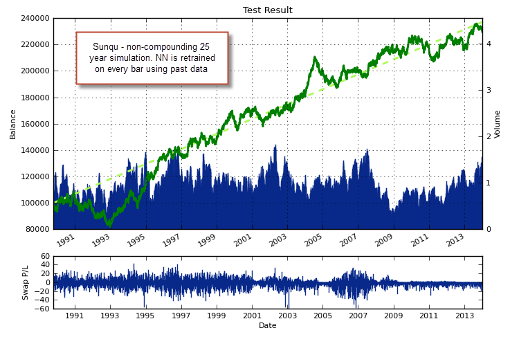
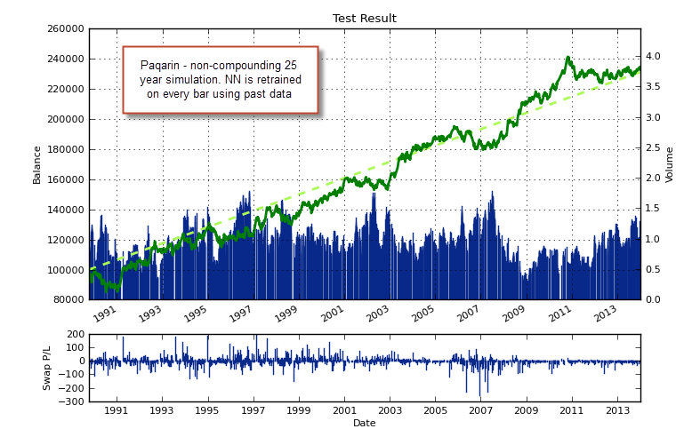
I have to confess that my quest to improve neural network trading strategies has been filled with frustration. It took me a long time to develop my first successful model (the Sunqu trading system — which is actually in profit after more than a year of live trading) but after this initial development I wasn’t able to improve it a lot further (beyond some small enhancements). After this I decided to leave this model alone – which is really complicated in nature – and attempt to develop a simpler model which would hopefully be easier to improve. This is when I developed the Paqarin system, which uses a simpler set of inputs and outputs in order to reach similar levels of historical profitability on the EUR/USD. However – to continue my frustration – Paqarin wasn’t very easy to improve as well. I did make some progress in improving this trading strategy during the last few weeks but I want to leave this discussion for a future post (as it deals with inputs).
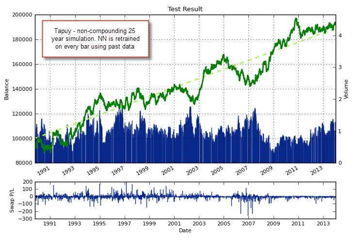
My last attempt to overcome the above problems was the Tapuy trading strategy, a system that was inspired on an article dealing with the use of NN on images. Using the ChartDirector, DeVil and FANN libraries I was able to implement an image creation and processing mechanism that used EUR/USD daily charts (a drastic reduction of them) to make predictions regarding the next trading day. This system is very interesting because it shows that the simple pixels within these graphics contain enough information as to make decisions that have a significant historical edge. Tapuy is also interesting in the sense that it processes trading charts, the same input that manual traders use to tackle the market. However this system was no panacea and improving this strategy was also extremely hard. Tapuy is also hard to back-test (takes very long due to the image creation and reading process) and therefore the amount of experiments that could be made was reduced.
After creating these three systems my new NN creations were nil. I couldn’t improve them substantially and I could not find a new strategy to create an NN, this was the main reason why I started to experiment with new machine learning techniques (such as linear classifiers, keltners, support vector machines, etc). However during last week I had a sort of epiphany when I was thinking about ways in which I could limit the market exposure of these systems by making them trade less in some manner and realized that the solution to my problems was in front of me the whole time. The solution to improve the performance of three classifiers – all of them showing long term historical edges – is simple… Just put them together to make trading decisions! :o)
–
–
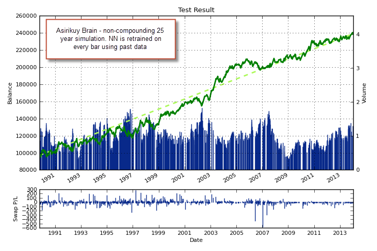
Surely my experience with other machine learning techniques told me that putting classifiers together to make trading decisions generally improved performance but I had never thought of putting these systems together because I viewed them mainly as separate trading strategies and not simply as machine learning decision makers. Nonetheless, it made perfect sense to put the three decision making cores into one strategy: what I now like to call the “AsirikuyBrain” and come to conclusions regarding trading decisions from a prediction that conforms to the three techniques. If they all have long term edges, then their total agreement should have more predictive power than their partial agreement. The result completely amazed me. The trading strategies improved each other’s statistics tremendously (much more than if they were traded together as systems within a portfolio) and moreover, they diminished the overall market exposure of the strategies by a big margin. The system only has one position open at any given time, but it needs all predictors to agree in order to enter or exit a position.
The overall profitability is the highest among all the systems and the drawdown is the lowest, this means that the AsirikuyBrain achieves an Average Annualized Return to Maximum Drawdown ratio that is higher than any of the individual trading techniques used, the maximum drawdown period length is also reduced considerably, from more than 1000 days for the other NN systems, to less than 750 days. The linearity of the trading system in non-compounding simulations also increases tremendously (to R^2 = 0.98), thanks to the smoothing power obtained from the committee effect (which means that the idea works!). As you can see on the images within this post, the curves for the individual systems are markedly inferior when compared with the equity curve of the AsirikuyBrain strategy. I will continue to make some tests and improvements, so expect some new posts on NN within the next few days and weeks (including some posts about inputs, prediction accuracy Vs profitability and predictions of profitability Vs predictions of directionality).
If you would like to learn more about neural network strategies and how you too can build constantly retraining NN systems using FANN that can be executed on MQL4/MQL5/JForex or the Oanda REST API, please consider joining Asirikuy.com, a website filled with educational videos, trading systems, development and a sound, honest and transparent approach towards automated trading in general . I hope you enjoyed this article ! :o)


Hi Daniel,
are you going to release this AsirikuyBrain ea in the near future?
best regards,
Rob.
Hi Rob,
Thanks for your comment :o) Yes, it will be on the F4.3.14 update next week-end,
Best regards,
Daniel
Interesting concept. I’m calculating a CAGR = 3.5% or near it. I think this is too low (SPX TR for same period is about 10%) and combined with the very long drawdown I think you may still have a long way to go with this. It is good you are persistent though.:)
What about if you adjust position size 2 predictions agree to 2/3 and size up to full position when they all agree?
Do you keep the position open until a predictor does not agree or you just close it at the end of the day? I don’t know if I missed that.
Hi Bob,
Thanks for posting :o)
The CAGR cannot be calculated from this non-compounding simulation as you would a regular one, since the risk is a constant amount in USD (1% of initial balance). When using regular money management (1% risk of balance on trade open) the CAGR is actually near 10% and the AAR/MaxDD is in the 0.8-0.9 region (maximum DD is about 13.5%). Regular compounding money management would generate exponential grow charts (which are hard to visually interpret properly) reason why I always post non-compounding simulations. However when trading live you would always use regular money management, risking a fixed percentage of the balance on trade open. Bishoftu I’ve also made some significant improvements within the last few days and have got the Max drawdown length under 500 days :o)
It’s an interesting idea! I’ll give it a try and see what I get.
I tried both, closing positions on some disagreement gave me worse results, I only close trades whenever the SL is hit or an opposite signal (where all NNs agree) appears.
Thanks again for commenting Bog :o)
Best Regards,
Daniel
“Regular compounding money management would generate exponential grow charts (which are hard to visually interpret properly) reason why I always post non-compounding simulations. However when trading live you would always use regular money management, risking a fixed percentage of the balance on trade open.”
I am of the opinion that regular MM should be used in backtests because it is a proper anti-martingale method. It is rare to see exponential growth due to drawdowns. The best way to backtest is I believe the way you actually trade and that involves MM.
Yes of course, I fully agree with that, this (with MM) is obviously the way in which we back-test systems to analyse before live trading. I only perform the non-compounding simulations on the blog because they’re easier to analyse and draw conclusions from (having only the charts). A regular MM simulation without the statistics (only the chart) is harder to analyze. Next time I’ll post some regular MM statistics as well. Thanks again for commenting Bob :o)
The linearity of the equity curve is very impressive Daniel. Thank you for sharing your hard work.
Regards
Rodney