The key to profitable trading under real out-of-sample (OS) conditions – meaning under data that didn’t exist when you created the strategy – is to be able to draw some type of predictions about which strategies will be better performing in the future. This means that you must have some idea about how the past characteristics of the system will relate with its future characteristics. I have discussed this several times in the past – read here and here – where it seems that in-sample (IS) return related statistical characteristics bear little or no relationship with future system characteristics, that is, a system’s in-sample back-testing sharpe, profit factor, etc have little to nothing to do with its statistics under real new market conditions. However I had also written a post related with pseudo out-of-sample tests – see here – where it was somewhat clear that although correlations would be low when systems started trading, there would be an increase in these correlations as the systems traded for longer periods of time. This week I wanted to put this hypothesis to the test using our PA repository’s IS and OS Sharpe and Profit Factor statistics.
–

–
It is certainly discouraging to look at a system’s Profit Factor or Sharpe ratio in back-tests and see that it really has nothing to do with what you got in live trading. When you have many systems and you try to see if there is any correlation and you see that there is none, then it becomes even more discouraging as it’s easy to think that you’re simply wasting your time by trying to generate systems that conformed to some performance benchmark in the past. What is the point of generating a system with a higher PF if higher PF in the IS does not mean a higher PF in the OS? Of course an important fact here is that we’re usually comparing a much longer IS with a much shorter OS, which means that things should be expected to be very different. It is certainly naive to think that the PF of a 2 month period will be proportional to the PF of a 30 year old period, a 2 month period is much more random and – just by looking at the distribution of PF values in the IS – it becomes clear that drawing any type of expectation that can be related in terms of a correlation is difficult.
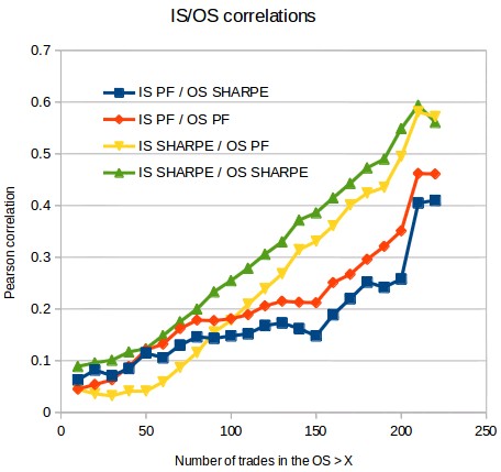
However once systems trade for longer they should show stronger and stronger IS/OS correlations if there is any influence of the IS period into the OS. That is, if there is some merit to selecting better systems in the IS then this should show as some type of correlation that increases in value as the OS grows longer. If no such correlation exists then the systems are hopeless victims of some type of statistical bias source (curve-fitting or data-mining bias to name the most difficult to eradicate) and the effort to filter strategies in the IS is meaningless. To put this to the test I used our PA repository – presently with more than 10K strategies – with some of these strategies now trading for more than 3 years under real OS conditions (meaning these market conditions didn’t exist when the systems were created).
–

–
The results in the first image of this post show that what we have is indeed a linearly increasing correlation, in line with my post on pseudo out-of-sample periods, of both the Sharpe and Profit Factor IS to OS values. As we go from all systems with more than 10 trades with systems with more than 220 trades the pearson correlations increase dramatically from near zero to more than 0.5 for systems with more than 220 trades. This relationship is very encouraging as the increase is faster than what was expected from pseudo out-of-sample testing. This might be because these p-OS tests did not include data-mining bias assessments which are key to eliminate an important source of bias that might make this evolution slower.
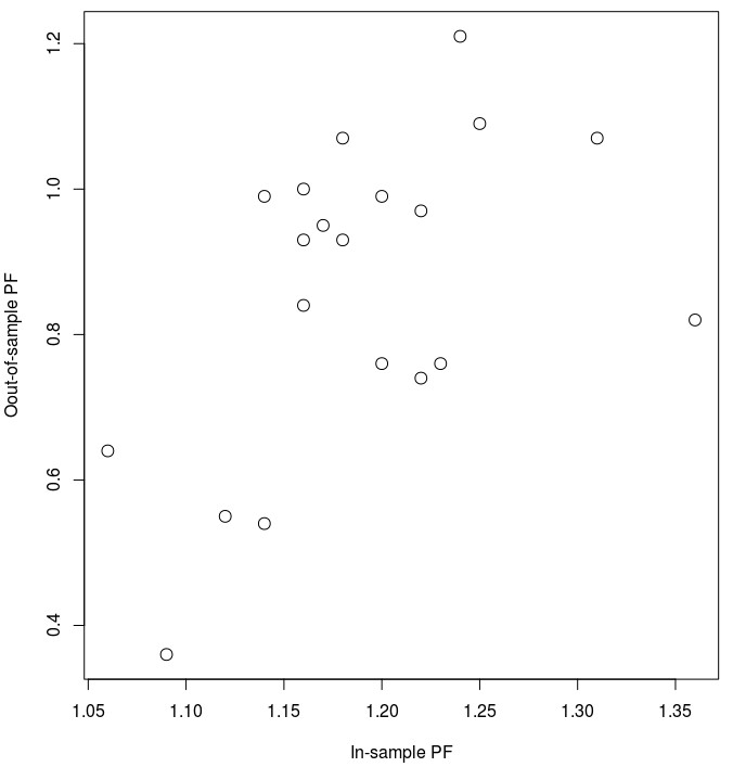
Of course it is also worth mentioning that correlation does not imply that the PF values are equivalent. The fact that IS/OS PF/Sharpe values become more correlated does not mean that a PF of 1.5 in the IS becomes a PF close to 1.5 in the OS, it just means that a higher overall PF in the IS is related with a higher PF in the OS but the correspondence – the slope of this relationship – is not one due to alpha decay. The second graph in this post shows you the IS and OS PF values for systems with more than 250 trades – where the correlation goes up to 0.50 for these variables (as it’s evident we don’t have many systems with so many trades in the OS). As you can see a PF of 1.20 does not immediately imply a PF of 1.20 in the OS but in this case having an IS PF of 1.25 actually implies that the created system’s OS performance is expected to be just close to BE.
–

–
The above results are very important because they point to the fact that IS mining of higher PF/Sharpe values makes sense because higher IS values do tend to lead to higher OS values for our systems. While the slope of this relationship is clearly less than 1 – due to alpha decay caused by changes in market conditions – the clear conclusion is that in the long term using the top IS performers of the Sharpe and Profit Factor variables should lead to better results than doing otherwise, a hypothesis that we’ll put to the test in live trading soon enough. As time passes and we obtain more data from our repository it will become possible for us to go deeper into this analysis and see how high the correlations really get as we move into longer and longer OS periods, so far the trend remains linear with no plateau in sight. If you would like to learn more about how you too can mine PA systems and trade our system repository with more than 10K systems please consider joining Asirikuy.com, a website filled with educational videos, trading systems, development and a sound, honest and transparent approach towards automated trading.


